Chapter 21 A Simple Linear Model

BuildIt Inc. flips houses - they buy houses to quickly renovate and then sell. Their specialty is building additions on to existing houses in established neighborhoods and then selling the home at prices above their total investment. BuildIt’s decision to move into a neighborhood is based on how sales price fluctuates with square footage. If sales price seems to increase by more than $120 per additional square foot, then they consider that neighborhood to be a good candidate for buying houses. BuildIt is eyeing a new neighborhood and records the square footage and prices of some recent sales transactions.
The following code creates a dataframe with BuildIt’s findings (note: salesPrice is in thousands of dollars):
library(tidyverse)
dataDF = tibble(
  salesPrice = c(160, 220, 190, 250, 290, 240),
  sqFootage = c(960, 1285, 1350, 1600, 1850, 1900))
Visually, we can confirm what appears to be a linear relationship between square footage and sales prices by creating a scatterplot with a linear regression line drawn in blue:
library(ggplot2)
dataDF %>%
  ggplot(aes(x = sqFootage, y = salesPrice)) +
  geom_point() +
  geom_smooth(method = "lm", se = FALSE)
Figure 21.1: The so-called best line fit to six points. It is the line that minimizes the squared deviations between the line’s predictions of price and the observed prices. We will seek to draw multiple plausible lines, not just one.
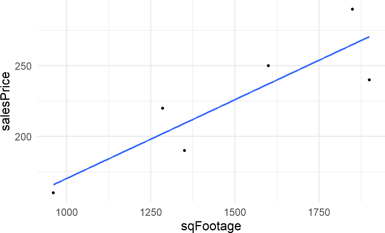
BuildIt is interested in the slope of this line which gives the estimated change in mean sales price for each unit change in square footage. For BuildIt, they want to know if this slope is above 120 per square foot?
Letting,
\[ \begin{aligned} x_i \equiv &\textrm{ The square footage for the } i^{th} \textrm{ house.} \\ y_i \equiv &\textrm{ The observed sales price, in 000's, for the } i^{th} \textrm{ house.} \\ \alpha &\equiv \textrm{ The intercept term for the regression line.} \\ \beta &\equiv \textrm{ The slope coefficient representing change in expected price per square footage.} \\ \mu_i \equiv &\textrm{ The expected sales price, in 000's, for any given square footage where } \\ & \hspace{0.2cm} \mu_i = E(y_i | x_i) \textrm{ and } \mu_i = \alpha + \beta \times x_i. \end{aligned} \]
the regression output can be extracted using the lm() function in R. \(\alpha\) is the (intercept) and sqFootage is the slope coefficient, \(\beta\), for square footage:
##
## Call:
## lm(formula = salesPrice ~ sqFootage, data = dataDF)
##
## Coefficients:
## (Intercept)    sqFootage
##     58.9064       0.1114
Based on the output, the following linear equation is the so-called “best” line:
\[ \mu_i = 58.91 + 0.1114 \times x_i \]
Using this model, BuildIt can anticipate being able to sell additional square footage for about $111 per square foot (i.e. \(1000* \beta\) because price is in 000’s). This would not earn them acceptable profit as it is less than $120 per square foot. However, with only 6 data points, there is obviously going to be tremendous uncertainty in this estimate. A Bayesian model can capture this uncertainty.
21.1 A Simple Bayesian Linear Model
From previous coursework, you are probably familiar with simple linear regression in a non-Bayesian context. Extending this model to our Bayesian context, we will create an observational model with the assumption that our observed data is normally distributed around some line. Let’s use the following notation to describe the line:
\[ \mu_i = \alpha + \beta x_i \]
where,
\[ \begin{aligned} x_i &\equiv \textrm{The value of an explanatory variable for the } i^{th} \textrm{ observation.} \\ \alpha &\equiv \textrm{ The intercept term for the line.} \\ \beta &\equiv \textrm{ The slope coefficient for the line.} \\ \mu_i &\equiv \textrm{ The expected value (or mean) for the } i^{th} \textrm{ observation.} \end{aligned} \]
In our generative DAG workflow, we represent the Bayesian version of simple linear regression:
library(causact)
graph = dag_create() %>%
  dag_node("Sales Price","y",
           rhs = normal(mu,sigma),
           data = dataDF$salesPrice) %>%
  dag_node("Expected Sales Price","mu",
           child = "y",
           rhs = alpha + beta * x) %>%
  dag_node("Intercept","alpha",
           child = "mu",
           rhs = uniform(-100,175)) %>%
  dag_node("Square Footage","x",
           data = dataDF$sqFootage,
           child = "mu") %>%
  dag_node("Price Std. Dev.","sigma",
           rhs = gamma(4,0.1),
           child = "y") %>%
  dag_node("Price Per SqFt Slope", "beta",
           rhs = normal(0.120,0.80),
           child = "mu") %>%
  dag_plate("Observations","i",
            nodeLabels = c("y","mu","x"))

graph %>% dag_render()
Figure 21.2: Generative DAG model using Bayesian linear regression.
The statistical model of the generative DAG in Figure 21.2 has reasonable priors that we will analyze later - for now, let’s digest the implied narrative. Starting at the bottom:
- Sales Price Node(
y): We observe Sales Price data where each realization is normally distributed about an Expected Sales Price, \(\mu\). - Expected Sales Price Node(
mu): Each realization \(\mu\) is actually a deterministic function of this node’s parents. Graphically, the double perimeter around the node signals this. This node’s presence on the observation plate alerts us that this expectation varies with each observation. The only way this can happen is that it has a parent that varies with each observation; namely Square Footage. - Square Footage Node(
x): The Square Footage is observed (as noted by the darker fill) and its lack ofrhsmeans we are not modelling any of the variation in realizations (\(x\)); we just take it as a given. - All other yet-to-be discussed nodes are outside the Observations plate. Therefore, the model assumes these three other nodes each have one true value. The one we are most interested in Price Per SqFt Slope, \(\beta\), as this will serve as an estimate of how home prices change when Build-It adds square footage. Intercept just sets some base-level home value and Price Std. Dev. gives a measure of how much home prices vary about the calculated expected price, \(\mu\).
A main deficiency of non-Bayesian linear regression lines is that they do not measure uncertainty in slope coefficients as well. Ultimately, we would rather make decisions that do not fall victim to the hubris of a single estimate and instead make informed decisions with measured uncertainty. For us, we seek to investigate all plausible parameter values for the square footage coefficient, not just one.
To highlight the idea of having multiple plausible lines, consider capturing the relationship between sales price and square footage using one of these 8 alternative lines (shown using dashed lines):
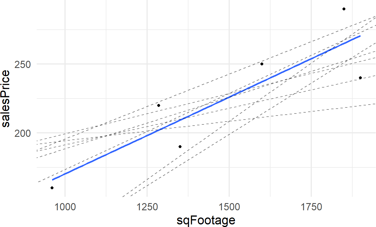
Might these alternative lines also describe the relationship between square footage and the expected sales price of a house? Actually, they do seem reasonable - by golly, there should be multiple plausible lines. So instead of just defining one plausible line, let’s use Bayesian inference to get a posterior distribution over all plausible lines consistent with our model.
Our interest is in the slope of the plausible lines. Because different slope terms can dramatically affect where the line crosses the y-axis, the intercept term should be allowed to fluctuate. Instead of trying the difficult task of placing a prior on the intercept, we can just use a wide uniform prior where we know the line will be positively sloped and not too far from 0. A better way to do this is to transform x to represent the deviation from the average x. In this case, the intercept prior just represents our belief about the price of an average square footage house. This is shown in the robust model of section 22.2.
To get our posterior, the numpyro model is executed with additional arguments so that it runs longer to yield the posterior distribution (extra samples are needed to explore the posterior realm because both our measly 6 points of data and our weak prior leave a very large plausible space to explore):
When analyzing the posterior distribution, we are really just interested in the slope coefficient (i.e. 000’s per square foot), we just want a posterior distribution over \(\beta\). Visually, that posterior distribution can be retrieved by
Figure 21.3: Posterior distribution for beta in BuildIt’s generative DAG.
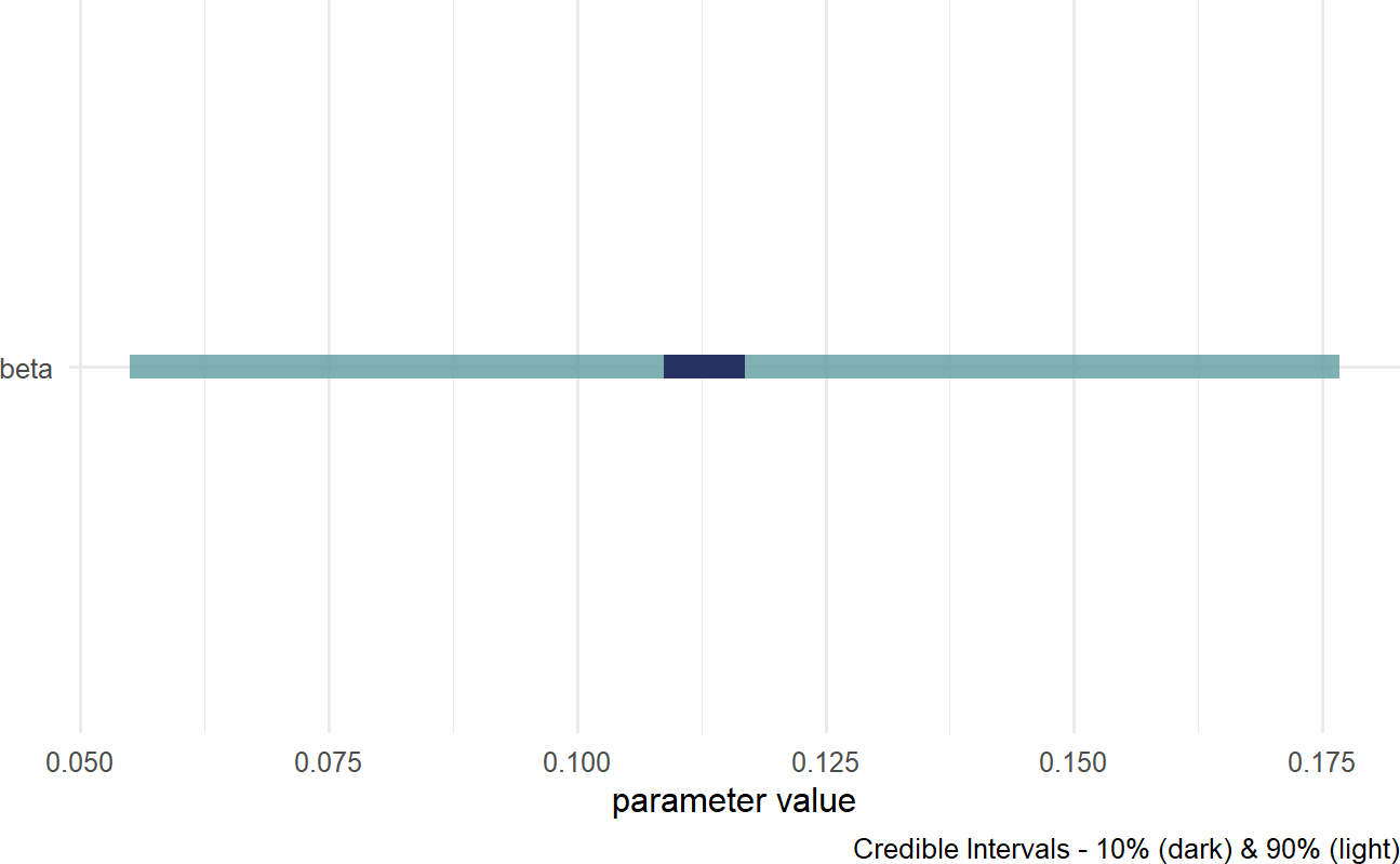
Figure 21.3 shows estimates around 0.120 are plausible, but does not clearly put the majority of plausibility above 0.120. While the estimates are most likely positive (most of the posterior density is where \(\beta>0\)), the percent above 0.120 will have to be calculated via a query of the posterior distribution:
## # A tibble: 1 × 1
##   pctAbove120
##         <dbl>
## 1       0.419
Yielding an approximate 41.9% probability for the company to at least break-even.
Interestingly, because of the uncertainty in the estimate, there is still meaningful probability that the company can earn much more than $120 per square foot, For example, here is the probability of being above $140 per square foot.
critValue = 0.140
drawsDF %>%
  mutate(aboveCriticalValue =
           ifelse(beta > critValue,1,0)) %>%
  summarize(pctAbove = mean(aboveCriticalValue))
## # A tibble: 1 × 1
## pctAbove
## <dbl>
## 1 0.219yielding an approximate 21.9% probability for the company to earn over a very favorable $140 per square foot.
Please note that many more factors influence home price than just square footage. This model is purely for education purposes and a more detailed generative DAG to include more factors driving real-estate prices is beyond the scope of this book. Please know that you are given the building blocks to pursue that DAG if you choose.
In conclusion, there is still alot of uncertainty in the estimate of \(\beta\). Yet, the company needs to make a decision. If all relevant information has already been collected and BuildIt wants to be confident they will not lose money, then the best decision is to not invest in houses from this neighborhood. However, given the uncertainty in the estimate, this neighborhood certainly has the potential to be profitable. More data and/or more modelling assumptions will be the only ways to reduce that uncertainty and hence, be more confident in this opportunity. This makes sense - we only have six data points to go off of.
21.2 Adding Robustness
When modelling, assumptions should reflect the reality you are trying to model. Use care traversing the business analytics bridge from real-world to math-world. For example, when it comes to housing prices, there might be alot of outliers in your data. Hence, it might be better to say that housing prices are \(\textrm{student-t}\) distributed about some expected sales price rather than normally distributed - this will make estimates much more robust to outliers. In a Bayesian context, model assumption changes are readily accomodated, we do not need new or special techniques. Figure 21.4 shows the generative DAG changing the observed data distribution from \(\textrm{normal}\) to \(\textrm{student-t}\).
library(causact)
graph = dag_create() %>%
  dag_node("Sales Price","y",
           rhs = student(nu,mu,sigma),  ###NEW DIST.
           data = dataDF$salesPrice) %>%
  dag_node("Deg. of Freedom","nu",    ###NEW NODE
           child = "y",
           rhs = gamma(2,0.1)) %>%
  dag_node("Expected Sales Price","mu",
           child = "y",
           rhs = alpha + beta * x) %>%
  dag_node("Price Std. Dev.","sigma",
           rhs = gamma(4,0.1),
           child = "y") %>%
  dag_node("Square Footage","x",
           data = dataDF$sqFootage,
           child = "mu") %>%
  dag_node("Intercept","alpha",
           child = "mu",
           rhs = uniform(-100,175)) %>%
  dag_node("Price Per SqFt Slope", "beta",
           rhs = normal(0.120,0.80),
           child = "mu") %>%
  dag_plate("Observations","i",
            nodeLabels = c("y","mu","x"))

graph %>% dag_render()
Figure 21.4: Generative DAG model using Bayesian linear regression.
21.3 Explanatory Variable Centering
There are always mathematical tricks to do something a little better. In this book, we mostly shy away from the tricks to focus on the core creation process of generative DAGs. However, as you advance on in your BAW journey, you’ll see models leveraging these tricks as if they are common knowledge.
Figure 21.5: Showing where the regression line (dark line) and two other plausbile lines (light lines) cross the y-axis. Note how far away this crossing is from any data. Houses tend to be of a minimum size and its meaningless to talk about sales prices of houses that have zero or small square footages.
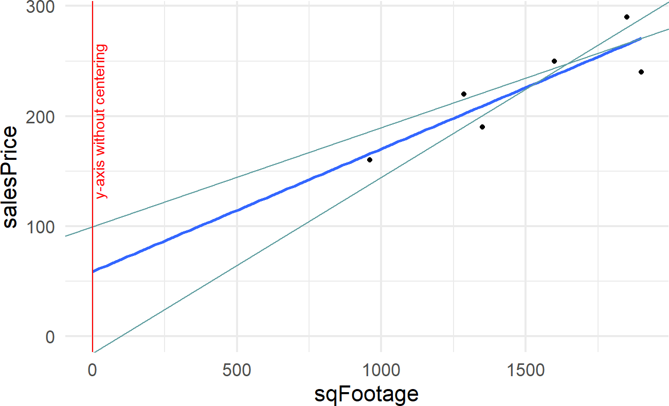
The trick we will use now is centering an explanatory variable. Figure 21.5 expands the regression line shown in Figure 21.1 to show the y-intercept at the point (0,58.9) and two other lines that plausibly describe the data. Notice the wild swings in intercepts of these lines. We captured knowledge about these wild swings with this node in Figure 21.6, but it does not feel natural.
Figure 21.6: The prior used for the intercept term.
After adding a centered column of square footage to dataDF:
We can create Figure 21.7:
dataDF %>%
  ggplot(aes(x = centeredSqFootage, y = salesPrice))  +
  geom_vline(xintercept = 0, color = "red") +
  geom_point() +
  geom_smooth(method = "lm",
              se = FALSE,
              fullrange = TRUE) +
  annotate("text",x = 20, y = 195,
           label = "new y-axis after centering",
           angle = 90, color = "red")
Figure 21.7: Regression line drawn after centering the explanatory variable. The slope of the line remains unchanged, but the y-intercept now reflects the sales price of an average house.
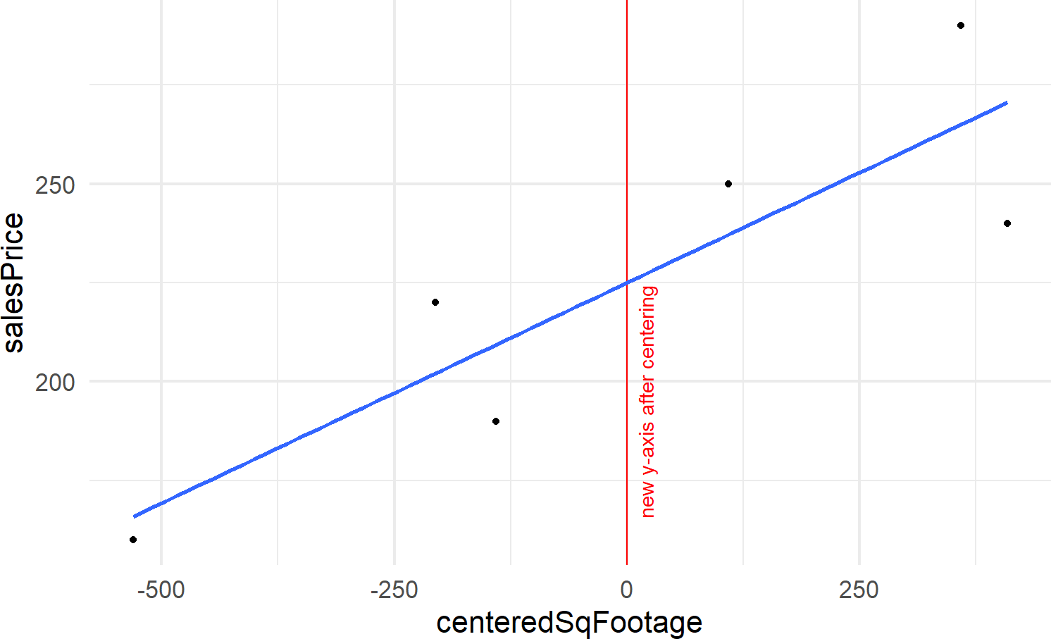
By centering the Square Footage variable, we are effectively shifting the y-axis to be drawn in the middle of our Square Footage data, \(x\). More importantly, this transforms our interpretation of the y-intercept. Any line predicting expected sales price now intersects the y-axis at the average square footage. Hence, our y-intercept is the expected sales price of an average house. It is much easier for us to elicit assumptions about the average price of an average house than it is to imagine the meaning of the y-intercept for a zero square foot house. For our problem, we will say the average house gets sold in the $200K range, \(\alpha \sim N(200,50)\). The updated generative DAG is shown in Figure 21.8.
graph = dag_create() %>%
  dag_node("Sales Price","y",
           rhs = student(nu,mu,sigma),
           data = dataDF$salesPrice) %>%
  dag_node("Deg. of Freedom","nu",
           child = "y",
           rhs = gamma(2,0.1)) %>%
  dag_node("Expected Sales Price","mu",
           child = "y",
           rhs = alpha + beta * x) %>%
  dag_node("Price Std. Dev.","sigma",
           rhs = gamma(4,0.1),
           child = "y") %>%
  dag_node("Cent. Square Footage","x",
           data = dataDF$centeredSqFootage, ## CHANGE
           child = "mu") %>%
  dag_node("Intercept","alpha",
           child = "mu",
           rhs = normal(200,50)) %>%  ## CHANGE PRIOR
  dag_node("Price Per SqFt Slope", "beta",
           rhs = normal(0.120,0.80),
           child = "mu") %>%
  dag_plate("Observations","i",
            nodeLabels = c("y","mu","x"))

graph %>% dag_render()
Figure 21.8: Generative DAG model using Bayesian linear regression with centered explanatory variable.
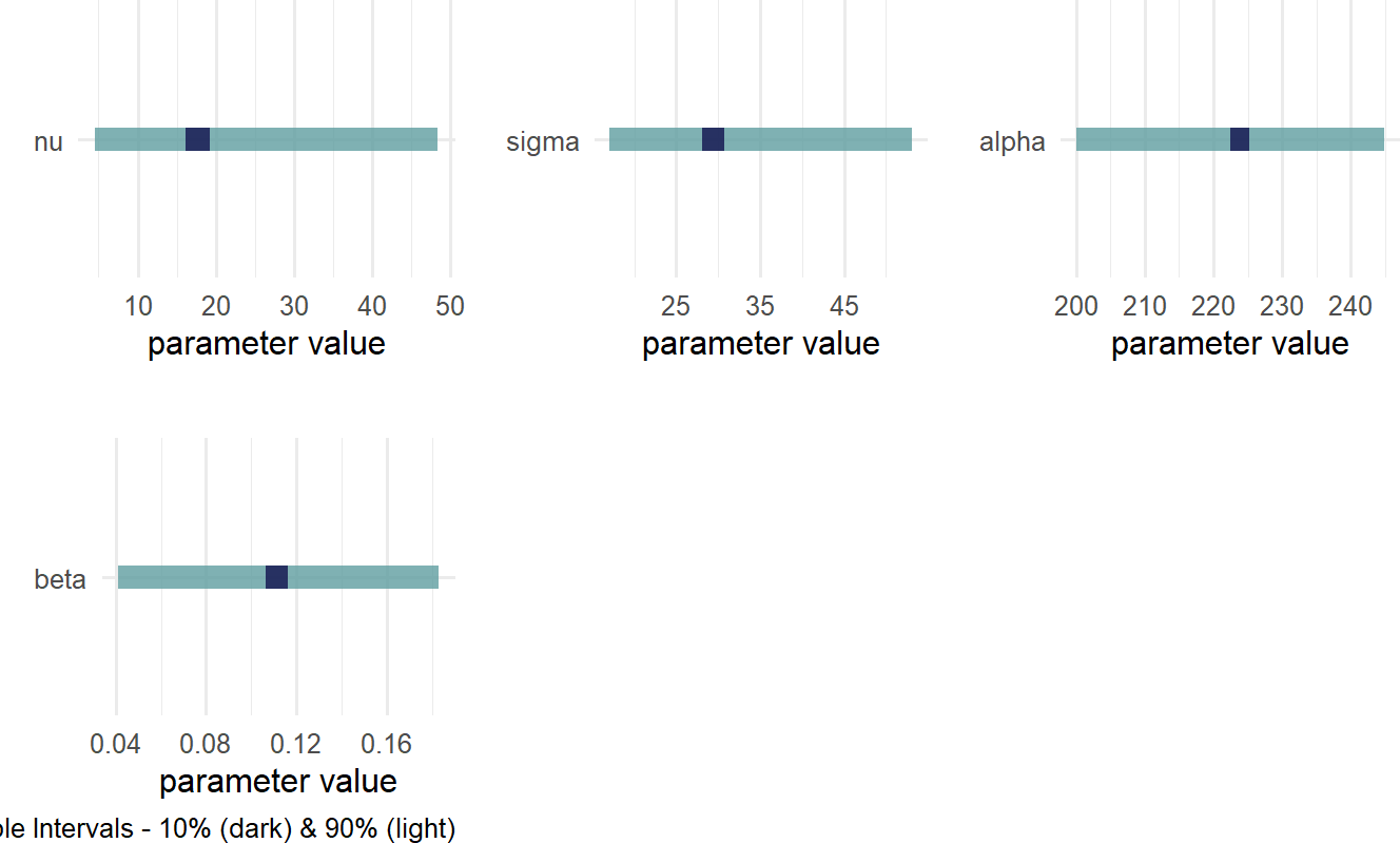
Retrieving the posterior distribution gives Figure 21.9.
Figure 21.9: Posterior distribution for a robust Bayesian linear regression with centered explanatory variable.
And doing a variation of a posterior predictive check, we plot a sample of plausible lines from the posterior against the observed data:
## get 20 draws from posterior
plotDF = drawsDF %>%
  slice_sample(n=20)

dataDF %>%
  ggplot(aes(x = centeredSqFootage, y = salesPrice)) +
  geom_point() +
  geom_smooth(method = "lm", se = FALSE) +
  geom_abline(data=plotDF,
              aes(intercept = alpha, slope = beta),
              alpha = 0.5,  # transparency arg.
              color = "cadetblue")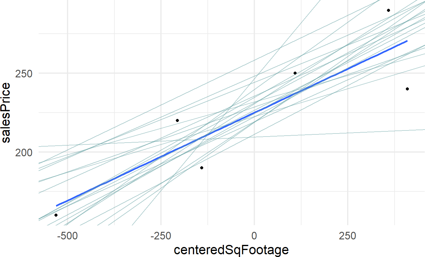
and realize that there are lots of lines that look plausible through our data. Build-it is going to need more data before they can be confident about the relationship between price and square footage.
21.3.1 Notes on thinking like a Bayesian
More generally, please start to think of Bayesian models as things you, as a Business Analyst, get to create. As long as you are mimicking reality with your models, you will find great success taking the building blocks you know and building models of increasing complexity that capture further nuances of the real-world. These models are yours to build - go boldly and make tailored models of the world you work in!
21.4 Getting More Help
Richard McElreath’s course uses Stan instead of causact and numpyro, yet outside of the computational engine, the material is relevant to your study. I highly recommend his lesson on linear models (see https://youtu.be/0biewTNUBP4). If you have the time, watch from the beginning. If you want to zero in on the simple linear model, he creates the first linear model trying to predict height as a function of weight at 43:00.
21.5 Exercises
For this chapter’s exercises, we look at 1,460 observations of home sales in Ames, Iowa. Let’s use this overly simplified generative model of housing prices to explore the interpretation of linear models. Here is the model we will use based on the houseDF data frame which is built into the causact package:
library(causact)
library(tidyverse)
## get avg salePrice to center explantory variable
meanSqFt = mean(houseDF$`1stFlrSF`)

## simplify dataframe to work with
salesPriceDF = houseDF %>%
  mutate(salePrice = SalePrice,
         sqFt = `1stFlrSF` - meanSqFt,
         area = Neighborhood) %>%
  select(salePrice, sqFt, area)

## model avg price and price per sq. foot by area
graph = dag_create() %>%
  dag_node("Sales Price","y",
           rhs = student(nu,mu,sigma),
           data = salesPriceDF$salePrice) %>%
  dag_node("Deg. of Freedom","nu",
           child = "y",
           rhs = gamma(2,0.1)) %>%
  dag_node("Expected Sales Price","mu",
           child = "y",
           rhs = alpha + beta * x) %>%
  dag_node("Price Std. Dev.","sigma",
           rhs = gamma(400,0.1),
           child = "y") %>%
  dag_node("Cent. Square Footage","x",
           data = salesPriceDF$sqFt,
           child = "mu") %>%
  dag_node("Intercept","alpha",
           child = "mu",
           rhs = normal(200000,50000)) %>%
  dag_node("Price Per SqFt Slope", "beta",
           rhs = normal(120,80),
           child = "mu") %>%
  dag_plate("Neighborhood","j",
            nodeLabels = c("alpha","beta"),
            data = salesPriceDF$area) %>%
  dag_plate("Observations","i",
            nodeLabels = c("y","mu","x"))

## report results
graph %>% dag_render()
Figure 21.10: A generative model for sales prices of homes in Ames, IA.
Assuming this generative model and the data it uses are representative of how housing prices work in Ames, IA; answer the following questions after generating and analyzing the posterior distribution.
Exercise 21.1 For an average-size home, which area would command the highest price? Do an Internet search (e.g. Zillow) for home sales in that area. Is your answer consistent with the prices you see on Zillow for Iowa home sales?
Exercise 21.2 What is the probability that an additional square foot added to a home in BrkSide is worth more than an additional square foot added to home in NoRidge?
Exercise 21.3 Investigate the area called Veenker. What might explain it having low alpha estimates and high beta estimates?