Chapter 13 Bayesian Inference On Graphical Models

13.1 An Illustrative Example

Figure 13.1: Before and after picture’s of Chili’s store remodelling initiative.

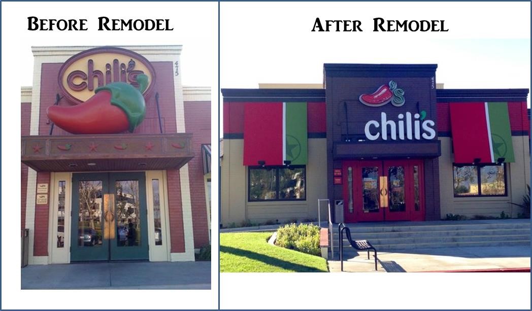
Figure 13.1 shows a sample of how Chili’s restaurants were refreshing their stores’ look and feel. You can imagine that through this investment Chili’s expects to increase store traffic. Let’s walk through a hypothetical argument between two managers as to the effect of this type of investment.

Assume the two managers have competing models for what effect a proposed Chili’s exterior remodel will have on its stores:

1. The Optimist Model (Model1) : This model is from a manager who is very excited about the effect of exterior renovations and argues that 70% of all Chili’s stores will see at least a 5% increase in sales.
2. The Pessimist Model (Model2) : This model is from a manager who felt the old facade was still fresh. This manager argues that only 20% of all Chili’s stores will see at least a 5% increase in sales.

These managers recognize and respect their differing opinions - they agree to test the remodel in a randomly chosen store. They hire you as a business data analyst and ask you to make the decision as to whose model is more right in light of the test’s results. Your job is to allocate credibility to the two competing models both before seeing results and after seeing results. Initially, you might not have any reason to favor one model over another, but as data is collected, your belief in whose model is more believable will change. For example, if the tested store sales decrease, then the pessimist model would seem more credible. Quantifying - using probability - how to allocate credibility both with and without data is your task.

13.2 Building A Graphical Model of the Real-World

The first step is to create a graphical model representation of the Chili’s question. Starting simple, let’s only imagine that we test the remodel in one store and our single data point (i.e. whether the one tested store increases sales or not) follows a Bernoulli distribution. The graphical model is simply the random variable oval:

And, the statistical model with the mathematical details is represented like this:

\[ \begin{aligned} X \equiv& \textrm{ Sales Increase: } \\ & \textrm{ If sales increase more than 5}\% \textrm{, then }X=1 \textrm{ otherwise, }X=0.\\ X \sim & \textrm{ Bernoulli}(\theta)\\ \end{aligned} \]

⊕You might notice that \(\theta\) is being used in place of \(p\) for describing the parameter of the Bernoulli Distribution. Often, mathematicians will use greek letters to describe distribution parameters and use regular (Latin) letters for data that is observable in the real-world (e.g. a sales increase). Sometimes, we will spell out theta or other greek letters because the computational world does not make the actual greek letters like \(\theta\) easy to work with. **We will explore the more realistic case of multiple and infinite possiblities for \(\theta\) in subsequent sections.

Great, we have seen this model before when representing coin flips. Our data is analogous to heads or tails of a coin flip. The data will be reduced to a zero or one for each store. If given \(\theta\), we could generate random sales data using rbern(n=1, prob=theta), but, we do not know \(\theta\); the reason we are looking at data is to answer the question: “what is \(\theta\)?”

From the managerial story above, \(\theta\) can only take on two values.\(^{**}\) In the optimistic model \(\theta=70\%\) and in the pessimistic model \(\theta=20\%\). So, we have two models of the world and are uncertain as to which one is correct. Without data, we have no reason to believe one manager over another, so \(P(\theta=70\%)=50\%\) and \(P(\theta=20\%)=50\%\) - i.e. each manager is equally likely to be correct. This is just like saying \(P(model1)=P(model2)=50\%\). Before any data is considered, this allocation of credibility assigning probability to all considered models is called the prior. The prior is the initial probability allocated among all the possible models.

⊕See https://youtu.be/nCRTuwCdmP0 for gaining some intuition about prior probabilities.

So now, we can more completely specify our data story using both a graphical and a statistical model with specified prior probabilities. The graphical model we would use to communicate with stakeholders is now two ovals representing our uncertainty in the probability of success and the observed sales increase (random variable math-labels for \(\Theta\) and \(X\) are included for extra clarity in connecting the graphical model and statistical model):

And, the statistical model is represented like this:

\[ \begin{aligned} X \equiv& \textrm{ Sales Increase: } \\ & \textrm{ If sales increase more than 5} \% \textrm{, then }X=1 \textrm{ otherwise, }X=0.\\ X \sim & \textrm{ Bernoulli}(\theta)\\ \Theta \equiv& \textrm{ Store Success Probability: } \\ \end{aligned} \]

\[ \Theta \sim \begin{array}{ccc} \textrm{Outcome } & \textrm{ Realization }(\theta) & f(\theta) \\ \hline Model1 & \textrm{ 70}\% & \textrm{ 50}\% \\ Model2 & \textrm{ 20}\% & \textrm{ 50}\% \\ \end{array} \]

⊕\(\Theta\) is the uppercase Greek letter for lowercase \(\theta\). Recall, we try to use uppercase letters for random variables and lowercase letters for their realizations.

where the prior probability distribution for \(\Theta\) is given in tabular form.

⊕\(\Theta\) is just capital \(\theta\). Remember we use capital letters, even capital Greek letters, to represent a random variable. Lowercase letters represent realizations or observations.)

⊕Two main classes of statistical models exist. A generative model can be used to generate random data as it gives a full probabilistic recipe (i.e. a joint distribution) for creating random data. In contrast, a discriminative model classifies or predicts without the ability to simulate all the random variables of the model.

Figure 13.3 and the accompanying statistical model represents a generative model. A crude definition of a generative model is that it is a recipe for simulating real-world data observations. In this case, simulating a single store’s success mimics a top-down reading of Figure 13.3:

1. Simulate a potential success probability by randomly picking, with equal probability, either the optimist (\(\theta = 70\%\)) or pessimist model (\(\theta = 20\%\)).
2. Simulate a store’s success by using the probability from (1) and generating a Bernoulli random variable with that probability of success (\(X \sim \textrm{Bernoulli}(\theta)\)).

We can easily show how to simulate an observation by writing code for the recipe in R:

library(causact) # for rbern function
set.seed(111) # to get the same random numbers

# Generate Which Manager Model is Correct
# Map theta = 70% to the number 1 and
# map theta = 20% to the number 0.
sampleModel = rbern(n=1, p = 0.5)
theta = ifelse(sampleModel == 1, 0.7, 0.2)

theta ## print the random value

## [1] 0.7

# Generate 20 sample stores for that theta
rbern(n = 20, p = theta)

##  [1] 0 1 1 1 1 1 1 1 1 1 1 1 1 1 1 1 0 1 1 1

KEY CONCEPT: Much of your subsequent work in this course will use this notion of generative models as recipes. You will 1) create generative models that serve as skeleton recipes - recipes with named probability distributions and unknown parameters - for how real-world data arises, and 2) inform models with data by reallocating plausibility to the recipe parameters that are most consistent with the data. In the above, had the value of theta been hidden from you, you would be able to guess it from the data; most of the 20 stores succeeded in the simulation.

A guiding principle for creating good generative models is that the generated data should mimic data that you, as a business data analyst, believe is plausible. If the generative model outputs implausible data in high frequency, then your model is not capturing the essence of the underlying data story; your modelling assumptions will need work. When the generative model seems correct in the absence of data, then data can feed the updating process (to be explored in Section 13.4) which sensibly reallocates prior probability so that model parameters that tend to generate data similar to the observed data are deemed more plausible.

13.3 From Model To Joint Distribution

The graphical model of Figure 13.3 shows that we have uncertainty about two related random variables: 1) Success Probability (\(\Theta\)) and 2) Sales Increase (\(X\)). Our assumption - built into our prior - is that one of our two models, \(\theta = 70\%\) or \(\theta = 20\%\), is correct.\(^{**}\) We are also confident about what collecting data from one store might yield: either a single success or a single failure in terms of the sales increase. Prior to collecting data, there are four combinations of model and data that are potential truths. Each combination’s prior plausibility, represented by \(a\%, b\%, c\%,\) and \(d\%\), are elements in the below table:

⊕\(^{**}\) This implicit assumption that one of the considered generative models is correct is sometimes referred to as the small world assumption. See this comparison by Richard McElreath of small world versus large world highlighting the implications of this assumption: https://youtu.be/WFv2vS8ESkk.

\[ \begin{array}{cc|cc} & & \textrm{ Possible} & \textrm{Models } \\ & & \theta = 70\% & \theta = 20\% \\ \hline \textrm{Possible} & \textit{Success} & a\% & b\% \\ \textrm{Data} & \textit{Failure} & c\% & d\% \end{array} \]

Prior to data collection, we know (based on assumptions) a few things must be true:

⊕If you are rusty on your defintion of conditional probability, take a moment to refresh yourself by viewing this set of videos from Khan Academy: https://www.khanacademy.org/math/statistics-probability/probability-library/conditional-probability-independence/v/calculating-conditional-probability.

1. One of the four scenarios must be true, thus \(a+b+c+d = 1\).
2. Equal probability is given to the possible models such that \(P(\theta = 70\%)=P(\theta = 20\%)=0.5\), thus \(a+c = b+d = 0.5\).
3. Assuming any model is true, then we know the conditional probability of success - i.e. \(P(Success|\theta = 70\%) = 70\%\) and \(P(Success|theta = 20\%) = 20\%\) (this is just the definition of \(\theta\)).
4. If we apply the definition of conditional probability - i.e. \(P(A \textrm{ and } B) = P(B) * P(A|B)\), we can define all the probabilities:
   1. \(a = P(\theta = 70\%) * P(Success|\theta = 70\%) = 50\% * 70\% = 1/2 * 7/10 = 7/20\)
   2. \(b = P(\theta = 20\%) * P(Success|\theta = 20\%) = 50\% * 20\% = 1/2 * 2/10 = 2/20\)
   3. \(c = P(\theta = 70\%) * P(Failure|\theta = 70\%) = 50\% * 30\% = 1/2 * 3/10 = 3/20\)
   4. \(d = P(\theta = 20\%) * P(Failure|\theta = 20\%) = 50\% * 80\% = 1/2 * 8/10 = 8/20\)
5. The marginal probability of success (i.e. the probabilty of success without reference to the model) is the sum of the first row’s elements: \(P(Success) = P(Success \textrm{ and } \theta = 70\%) + P(Success \textrm{ and } \theta = 20\%) = a + b = 7/20 + 2/20 = 9/20\).
6. The marginal probability of failure (i.e. the probabilty of failure without reference to the model) is the sum of the second row’s elements: \(P(Failure) = P(Failure \textrm{ and } \theta = 70\%) + P(Failure \textrm{ and } \theta = 20\%) = c + d = 3/20 + 8/20 = 11/20\).

Taken together, the above truths enable us to fully specify the marginal distributions \(P(Model)\) and \(P(Data)\), as well as the joint distribution \(P(Model \textrm{ and } Data)\):

\[ \begin{array}{cc|cc|c} & & \textrm{ Possible} & \textrm{Models } & \textbf{} \\ & & \theta = 70\% & \theta = 20\% & P(Data) \\ \hline \textrm{Possible} & \textit{Success} & 7/20 & 2/20 & 9/20 \\ \textrm{Data} & \textit{Failure} & 3/20 & 8/20 & 11/20 \\ \hline \textbf{} & P(Model) & 10/20 & 10/20 & 20/20 \\ \end{array} \]

⊕When you see something like \(P(Model)\) or \(P(Data)\) what this really means is that if I specify a model (or data), you are able to return a probability. For example, \(P(\theta = 70\%) = 50\%\) and \(P(Success) = 9/20)\). These are called marginal distributions (literally because they are often calculated in the margins by summing rows or columns of a two-way table). Often, we are interested in the distribution over several random variables. This distribution is referred to as a joint distribution over those random variables. In our example, the joint distribution is represented as \(P(Model \textrm{ and } Data)\). This means if I give you any specific realizations of both \(Model\) and \(Data\), you can return a probability. For example, \(P(\theta = 70\% \textrm{ and } Success) = 7/20\).

In data analysis, we are always intereseted in updating our beliefs about \(P(Model)\). Right now, both models are allocated \(50\%\) plausibility, but as soon as we see a success or failure, we will want to reallocate that plausibility towards either the optimist model in the case of success or the pessimist model in the case of failure.

13.4 Bayesian Updating Of The Joint Distribution

Our generative model recipe led us to this prior joint distribution for \(P(Model \textrm{ and } Data)\):

\[ \begin{array}{cc|cc} & & \textrm{ Possible} & \textrm{Models } \\ & & \theta = 70\% & \theta = 20\% \\ \hline \textrm{Possible} & \textit{Success} & 7/20 & 2/20 \\ \textrm{Data} & \textit{Failure} & 3/20 & 8/20 \\ \end{array} \]

Inference is the process of reallocating prior probability in models based on observed data, i.e. determining \(P(model|data)\). Mathematically, there is only one way to do this- Bayes rule.

13.5 Inference Summary So Far

The steps for initially allocating and then, reallocating probability in light of data are to:

1. Make A Graphical Model - Construct plausible relationships among the inter-related random variables of interest - in this chapter’s example the two random variables were \(Success \textrm{ }Probability\) and \(Sales \textrm{ }Increase\).
2. Provide Prior Probabilities Via A Statistical Model - Create prior probabilities to ensure that your model can generate seemingly plausible data. Our prior was easy to figure out (50%/50%) based on the context, but in future chapters we will explore more complex scenarios.
3. Update Using Bayes Rule - Use Bayesian updating to process data and reallocate probability among the competing models. So far, we learned to do this mathematically, but we will leverage the power of R and its packages to make the computer do this tedious work for us.

⊕When additional data is received, please know that Bayes rule still works. Just take the posterior output from the original data, and then use that as your prior when digesting the new information. Equivalently, you can just update the original prior with the combined set of original data and new data. Either way, Bayes rule will yield the same results.

While the math may seem tedious now, we are actually learning the math now to move away from it in the future; once we understand how the math works, we can leverage computation to do the math for us with a deeper understanding of what the computation does.

13.6 Exercises

The code models the Chili’s restaurant example as seen in the chapter. A version of the example is repeated here for convenience:

Let us assume we have two competing models for what effect a proposed Chili’s exterior remodel will have on its stores. One manager is very excited about the effect of exterior renovations and argues that 70% of all Chili’s stores will see at least a 5% increase in sales. Let’s define some notation; the probability of seeing an increase of 5% in sales at any one store is \(\theta\) and for this optimistic manager \(\theta = 70\%\). Another manager argues that the old façade was not really dated and felt that only 20% of remodeled stores will see at least a 5% increase in sales, i.e. \(\theta = 20\%\). As a compromise, the managers agree to roll the renovation out to 20 randomly selected stores and then decide whether to remodel all the stores or wait to remodel the other stores. They elect you to make the decision as to who is right.

RUN THE CODE LINE-BY-LINE AND DIGEST WHAT HAPPENS WITH EACH LINE. CONFIRM THAT THE FINAL PLOT ECHOES THE MATH DONE FOR THE EXAMPLE AS PRESENTED IN THE CHAPTER. THEN, MODIFY THE CODE TO ACCOMMODATE THE FOLLOWING CHANGES TO THE BUSINESS ASSUMPTIONS:

• Assume a prior that gives equal weight to all managers’ models.
  
• Assume that you are interested in comparing more than just the two candidates Modify the code to compare 8 potential values: \(\theta \in \{0.1,0.2,0.3,0.4,0.5,0.6,0.7,0.8\}\).
• Assume that you collect data from FIVE stores. The first, second, and third stores’ sales did increase by over 5% and the fourth and fifth stores’ sales did not. For coding purposes, assume that a coin flip of heads represents success (i.e. store sales increased by 5% or more) and tails represents a failure (i.e. store sales did not increase).

From your graph of the posterior distribution, what value for \(\theta\) seems most likely (i.e. is the highest)? Enter your answer with one decimal place.

• Assume a prior that gives unequal weight to all managers’ models. Assume the most pessimistic manager who’s \(\theta = 10\%\) insists the prior on his belief to be 65% such that \(P(\theta = 10\%) = 65\%\). All other potential models get \(5\%\) prior probability each.
• Assume that you are interested in comparing more than just the two candidates Modify the code to compare 8 potential values: \(\theta \in \{0.1,0.2,0.3,0.4,0.5,0.6,0.7,0.8\}\).
• Assume that you collect data from SEVEN stores. The first, second, third, and fourth stores’ sales did increase by over 5% and the fifth, sixth, and seventh stores’ sales did not. For coding purposes, assume that a coin flip of heads represents success (i.e. store sales increased by 5% or more) and tails represents a failure (i.e. store sales did not increase).

From extracting the proper numbers from the vector of posterior probabilities, find the posterior probability \(P(\theta = 10\% | Data =4 success, 3 failures)\).