Chapter 24 Compelling Decisions and Actions Under Uncertainty
Figure 24.1: The posterior distribution from this generative DAG gives us a way of modelling uncertainty in the parameters we care about.
We now continue last chapter’s investigation of Crossfit Gym’s use of yoga. Our goal is to bring the mathematical estimates of our posterior distribution’s parameters back into the real-world with compelling and visually-based recommendations. To do this, we 1) define our outcomes of interest, 2) compute a posterior distribution for those outcomes, and 3) communicate our beliefs about those outcomes by visualizing the outcomes of interest.
24.1 Outcomes of Interest
Our main outcome of interest is signup probability. We will investigate signup probability by investigating that particular node in relation to our decision. Representing this is the deceptively simple generative decision DAG shown in Figure 24.2.
dag_create() %>%
  dag_node("Yoga Stretching?","yoga",
           dec = TRUE) %>%
  dag_node("Signup Probability","prob") %>%
  dag_edge("yoga","prob") %>%
  dag_plate("Stretch Type","",
            nodeLabels = c("yoga","prob")) %>%
  dag_render(shortLabel = TRUE, wrapWidth = 12)
Figure 24.2: Generative decision dag showing our interest in how yoga strecthing effects signup probability. The plate around the two nodes indicates we are investigating signup probability for each possible value of yoga stretching.
The top-down narrative of Figure 24.2 is as follows. Crossfit Gyms decides on whether to offer yoga stretching and the sign-up probability across their gyms changes as a result. Our job is to quantify this change and form an opinion on whether to offer yoga stretching or not across the gyms; we will form our opinion using the posterior distribution.
24.2 Computing Posterior Distributions for Outcomes of Interest
The last model in the previous chapter gets us the generative DAG of Figure 24.1. Running it through the dag_numpyro() function yields a posterior distribution, but our job as analysts is not over. We now have to make sense of the posterior distribution and communicate its implications to stakeholders.
Rerun the analysis at the end of the previous chapter concluding with:
where drawsDF is a representative sample of the posterior distribution associated with Figure 24.1. This data frame is a sample of 4,000 draws of 28 variables. Let’s list the 28 variables using names(drawsDF).
alpha_1 |
alpha_8 |
beta_3 |
beta_10 |
alpha_2 |
alpha_9 |
beta_4 |
beta_11 |
alpha_3 |
alpha_10 |
beta_5 |
beta_12 |
alpha_4 |
alpha_11 |
beta_6 |
mu_alpha |
alpha_5 |
alpha_12 |
beta_7 |
mu_beta |
alpha_6 |
beta_1 |
beta_8 |
sd_alpha |
alpha_7 |
beta_2 |
beta_9 |
sd_beta |
Figure 24.3 is a subset of Figure 24.1 and our objective node, theta (a.k.a. Signup Probability), is the last descendant or bottom-child node of the graph.** ** We safely omit the children of this variable to save space since they do not affect our decision. Perusing our posterior’s 28 random variables, we might notice that theta is not one of them. Bummer! We are going to need to do some coding to get a representative sample for theta.
theta is omitted because it is a calculated node; its realization is a deterministic function of its parent y which is also a calculated node. Note that an oval’s double-perimeter is the visual clue for a calculated node (see Figure 24.3). Its parents include both random and observed nodes. So to actually determine theta, we need follow the generative recipe from grandparents (alpha,beta,j, and x) to grandchild (theta) via linear predictor y.
Figure 24.3: The posterior distribution from this generative DAG gives us a way of modelling uncertainty in the parameters we care about.
Notice, we do not care about mu_alpha and the other parents of alpha and beta. Once we have a representative sample of alpha and beta, plus the observed nodes j and x , then we can calculate theta.
For example, let’s estimate the additional sign-up probability when using “Yoga Stretch” at gym number 12?
Get a single draw of the required nodes from the representative sample.
Compute a value for the linear predictor with and without yoga (i.e.
x=1andx=0, respectively) using the formula shown for this node in Figure 24.3. Plugging in forx, we get the two different values of linear preditorythat interest us:x=1\(\rightarrow y_{yoga} = \alpha_{12}+\beta_{12}*1\)) and without yoga (x=0\(\rightarrow y_{trad} = \alpha_{12}+\beta_{12}*0 = \alpha_{12}\)):Compute the values for
thetawith and without yoga at gym12 using the inverse-logit function (i.e. the link function formula shown for this node in Figure 24.3):Compute the increased probability of signup when using yoga at gym12:
And now, viewing these computed values:
## # A tibble: 1 × 7
##   alpha_12 beta_12 y_yoga y_trad theta_yoga theta_trad probIncDueToYoga
##      <dbl>   <dbl>  <dbl>  <dbl>      <dbl>      <dbl>            <dbl>
## 1    -1.74   0.428  -1.32  -1.74      0.211      0.149           0.0627
we see that for this draw, around 21% of yoga trial customers end up signing up for a membership versus 15% of customers doing traditional stretching. According to this draw then, approximately 6% is the signup probability increase due to yoga stretching.
Let’s get a little mathematical and declare this difference in probabilities to be a new random variable Z_{gymID} like:
\[ Z_{12} \equiv \textrm{ Probability increase due to yoga stretching at gym 12}, \]
The following code scales the above four steps for creating one draw to creating a column of representative samples for \(Z_{12}\):
postDF = drawsDF %>%
  select(alpha_12,beta_12) %>%
  mutate(y_yoga = alpha_12 + beta_12 * 1) %>%
  mutate(y_trad = alpha_12) %>%
  mutate(theta_yoga = 1 / (1+exp(-y_yoga))) %>%
  mutate(theta_trad = 1 / (1+exp(-y_trad))) %>%
  mutate(z_12 = theta_yoga - theta_trad)
The column we just made, z_12, is our posterior distribution for the change in probability due to yoga stretching. We can visualize and summarize this posterior density:
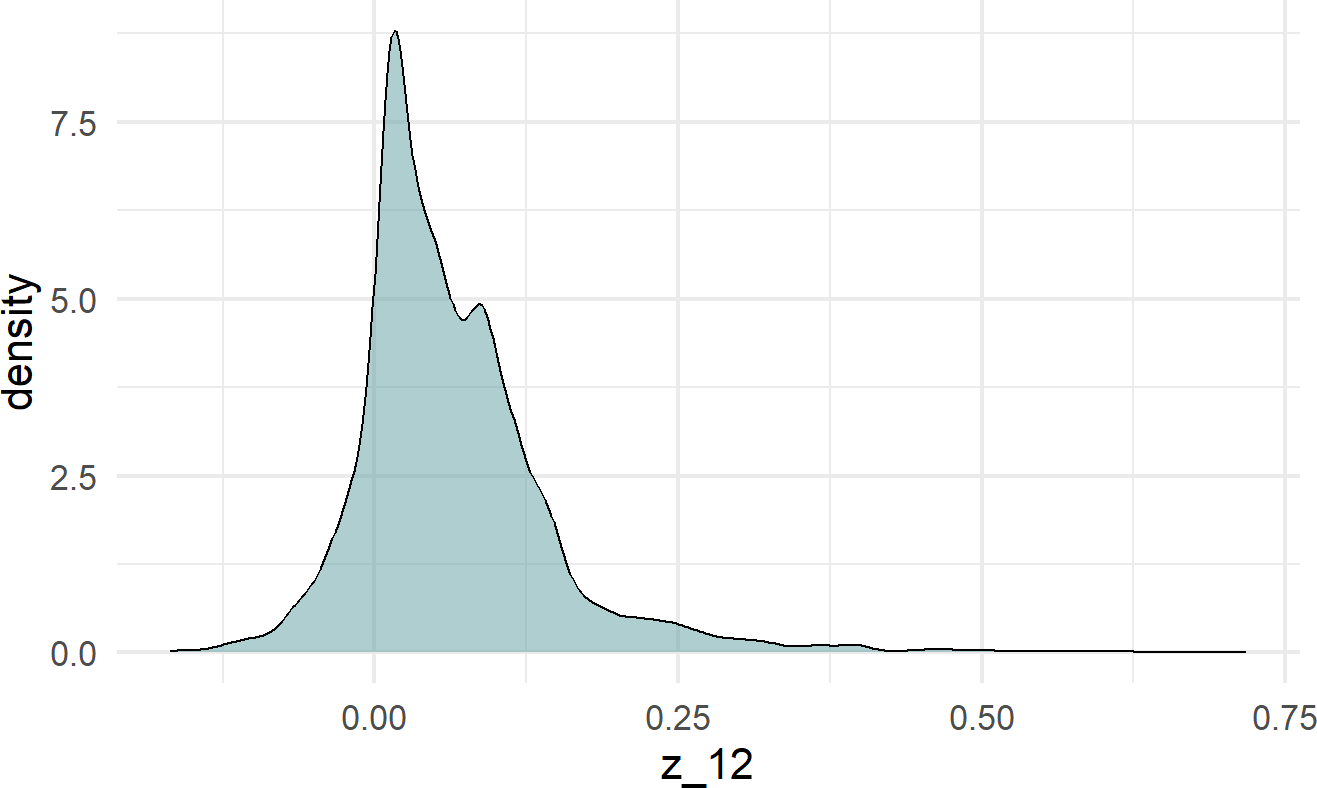
##     Min.  1st Qu.   Median     Mean  3rd Qu.     Max.
## -0.16815  0.01373  0.04783  0.06377  0.09554  0.71822
and form only a mild opinion that yoga is probably helpful at gym 12 (i.e. most of the plausible values are above zero).
24.3 Visual Advocacy for Decisions Which Improve Outcomes Of Interest
To convert posterior probabilities into decisions, we want a visual that communicates a recommendation. In business, a random variable outcome of interest is usually made more compelling by converting it to some measure of money. Let’s assume that that the value of each new customer is estimated to be $500 in net present value terms. We can then create a mathematical formula for value created by yoga stretching per trial customer:
\[ ValueOfYogaStretchingForGym12 = 500 \times Z_{12} \]
and also, represent it computationally
We now have a random variable of the per customer profit estimate if gym12 adopts yoga stretching for the next year versus not adopting yoga stretching. We can summarize this random variable graphically,
moneyDF %>%
  ggplot(aes(x = ValueCreated)) +
  geom_density(fill = "cadetblue", alpha = 0.5) +
  scale_x_continuous(labels = scales::dollar)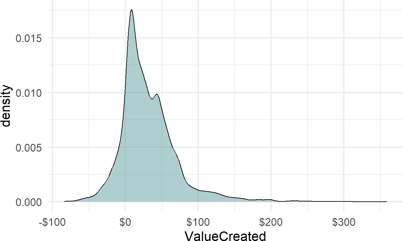
which shows both the plausibility of losing money as well as making up to say $100 per customer as a result of the decision. We can find some additional metrics:
##    Min. 1st Qu.  Median    Mean 3rd Qu.    Max.
## -84.077   6.865  23.914  31.884  47.769 359.112
telling us the median value for gym12 is about $24 of extra value per customer. This means that we assign a 50/50 chance to being above or below this number in terms of value created per customer. Hence, if it costs extra money (e.g. licensing fees, additional labor expense, additional equipment expense, etc.), say $25 per customer to offer the class, then this investment at gym12 might not be recovered.
Lastly, since continuous probability estimates are sometimes difficult for decision makers (and ourselves) to understand, we can create a discrete probability distribution by creating bins (see http://wilkelab.org/classes/SDS348/2016_spring/projects/project1/project1_hints.html).
breaks = c(-1000,-20,0,20,40,60,80,100,1000)
labels = c("<-$20","-$20 - $0","$0 - $20",
           "$20 - 40$","$40 - $60","$60 - $80",
           "$80-$100","$100+")
bins = cut(moneyDF$ValueCreated,
           breaks,
           include.lowest = T,
           right=FALSE,
           labels=labels)
moneyDF$bins = bins  ## add new column
And then, we use the newly created bins to give us a very nice and interpretable plot as shown in Figure 24.4.
## add label for percentage in each bin
plotDF = moneyDF %>%
  group_by(bins) %>%
  summarize(countInBin = n()) %>%
  mutate(pctInBin = countInBin / sum(countInBin)) %>%
  mutate(label = paste0(round(100*pctInBin,0),"%")) %>%
  mutate(makeMoney = ifelse(bins %in% levels(bins)[1:2],
                            "Not Profitable",
                            "Profitable"))

## Create more interpretable plot
plotDF %>%
  ggplot(aes(x = bins, y = pctInBin,
             fill = makeMoney)) +
  geom_col(color = "black") +
  geom_text(aes(label=label), nudge_y = 0.015) +
  xlab("Value Added Per Trial Customer") +
  ylab("Probability of Outcome") +
  scale_fill_manual(values = c("lightcoral",
                               "cadetblue")) +
  theme(legend.position = "none") +
  coord_flip() +
  ggtitle("Making Yoga Stretching Mandatory for Gym 12")
Figure 24.4: A More Interpretable Plot For Showing Potential Outcomes of The Policy.
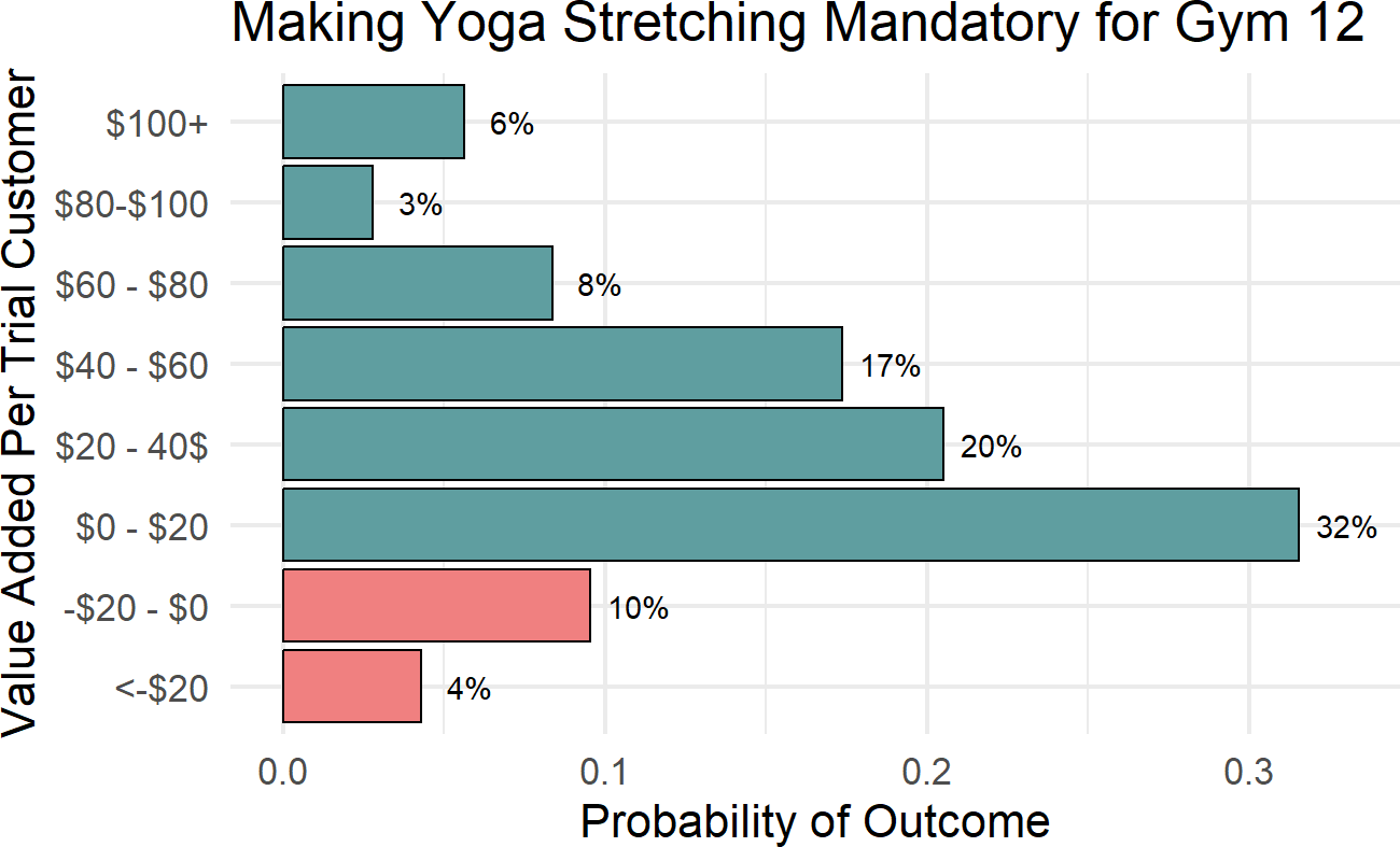
From the above, we can easily talk to any decision maker about the possiblities for various outcomes. For example, summing the bottom two percentages tells us there is an approximately 14% chance of yoga stretching creating negative value. Additionally, if Crossfit anticipates a cost of $20 per customer, then there is a 46% chance of not breaking even by using this policy.
24.4 Exercises
For this chapter’s exercises, we further examine the gymDF dataset of this chapter. Here is the model you should use to answer all exercises:
library(causact)
graph = dag_create() %>%
  dag_node("Number of Signups","k",
           rhs = binomial(nTrials,theta),
           data = gymDF$nSigned) %>%
  dag_node("Signup Probability","theta",
           child = "k",
           rhs = 1 / (1+exp(-y))) %>%
  dag_node("Number of Trials","nTrials",
           child = "k",
           data = gymDF$nTrialCustomers) %>%
  dag_node("Linear Predictor","y",
           rhs = alpha + beta * x,
           child = "theta") %>%
  dag_node("Yoga Stretch Flag","x",
           data = gymDF$yogaStretch,
           child = "y") %>%
  dag_node("Gym Intercept","alpha",
           rhs = normal(mu_alpha,sd_alpha),
           child = "y") %>%
  dag_node("Gym Yoga Slope Coeff","beta",
           rhs = normal(mu_beta,sd_beta),
           child = "y") %>%
  dag_node("Avg Crossfit Intercept","mu_alpha",
           rhs = normal(-1,1.5),
           child = "alpha") %>%
  dag_node("Avg Crossfit Yoga Slope","mu_beta",
           rhs = normal(0,0.75),
           child = "beta") %>%
  dag_node("SD Crossfit Intercept","sd_alpha",
           rhs = uniform(0,3),
           child = "alpha") %>%
  dag_node("SD Crossfit Yoga Slope","sd_beta",
           rhs = uniform(0,1.5),
           child = "beta") %>%
  dag_plate("Gym","j",
            nodeLabels = c("alpha","beta"),
            data = gymDF$gymID,
            addDataNode = TRUE) %>%
  dag_plate("Observation","i",
            nodeLabels = c("k","x","j",
                           "nTrials","theta","y"))
graph %>% dag_render()
Figure 23.15: A multi-level model of gym performance.
Exercise 24.1 In this chapter, we analyzed the monetary decision for gym12. Let’s now look at the implications of making yoga stretching mandatory for all new gyms. To do this, you would look at posterior estimates for \(\beta\) and \(\alpha\) - i.e. the parent nodes of \(\beta_j\) and \(\alpha_j\). These higher level estimates can be used to spawn new gyms with the \(\beta_j\) and \(\alpha_j\) drawn as random values from the \(\beta\) and \(\alpha\) distributions. Assuming it costs $10 extra for each trial customer to offer yoga stretching and that the value of a customer is $500, what is the probability that this mandatory yoga stretching policy is value creating for the Crossfit Gyms corporation?