Chapter 7 dplyr: Data Manipulation For Insight
I just got word that the CEO of ZappTech is thinking about hiring our consulting firm. Apparently, his category managers are refusing to talk to one another; acting as if the four product categories are isolated kingdoms.
Figure 7.1: Are ZappTech’s product categories providing the same service level for their customers?

He is convinced that ZappTech’s customers shop across multiple categories and thinks they expect the same level of customer service regardless of the product categories represented on their order. Since he doesn’t trust his own team to put effort towards integrating management of the categories, the CEO has provided us data and asked us to investigate two questions: 1) Does service level (measured by on-time shipments) vary across product categories? and 2) how often do orders include products from more than one product category.
We will use provided data (available from the causact package) to answer the CEO’s questions. In the process, we will learn more about data manipulation. The previous chapter presented tidy data frames as the starting point for data manipulation. In this chapter, the data is given in a slightly less than ideal format - we will learn to overcome this hurdle with some computational tricks, further exploring dplyr functions, and introducing the lubridate package for working with dates/times.
To answer the CEO’s questions, we will approach the data analysis in four phases:
- Data Loading: Make the data available in an data frame with all columns associated with the correct column class Commonly used column classes include character, numeric, integer, and date.
- Lateness Calculation: In this phase, we will learn about the
lubridatepackage in R and more rigorously define how to measure lateness. - Bring in product category information: In this phase, we will learn to merge the delivery information with the product category information using the join capabilities of dplyr.
- Answer the CEO’s questions: Does service level vary by product category? Do we ship items from multiple product categories?
7.1 Data Loading and Cleaning
Data loading begins by getting the data into your R environment. Since the data is built into the causact package, we just need to load the package and then access the data.
Two very common data file formats in which data is exchanged are
comma-delimited files (.csv) and Microsoft Excel files
(.xlsx). For importing and exporting .csv
files, use the read_csv() and write_csv()
functions from the readr package. For Excel files use the
read_excel() and write_excel functions from
the readxl package. Both packages are part of the tidyverse
collection of packages (https://www.tidyverse.org/packages/).
Remember, to install the causact and
lubridate packages if you have not done so already.
The data from the CEO is in two data frames built into the causact package that accompanies this book: delivDF and prodLineDF. The following command will load the delivDF data into your environment.
# make the causact package available in this R session
library("causact")

# uncomment THE below line to show datasets that
# are part of the causact package

# data(package = "causact") # uncomment for dataset list

# load/unhide the dataset from the causact package
data("delivDF")
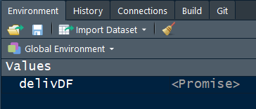 Figure 7.2: The delivDF dataframe details are not shown yet. The
 <promise> is an indication that once you try to use this R object, then and only then, will R load the object into the environment.
Figure 7.2 shows the updated environment tab in RStudio after running the above. Notice that it remains unclear what is contained within the delivDF data frame; the <Promise> description feels incomplete. This is due to something called lazy loading which refrains from completely loading the object into memory until the object is used. Thus, to see the details of delivDF, we just need to use it somehow. One way is to access the object by name - which prints the object to the console pane:
## # A tibble: 117,790 × 5
##    shipID plannedShipDate actualShipDate partID      quantity
##    <chr>  <chr>           <chr>          <chr>          <int>
##  1 10001  11/6/2013       10/4/2013      part92b16c5        6
##  2 10002  10/15/2013      10/4/2013      part66983b         2
##  3 10003  10/25/2013      10/7/2013      part8e36f25        1
##  4 10004  10/14/2013      10/8/2013      part30f5de0        1
##  5 10005  10/14/2013      10/8/2013      part9d64d35        6
##  6 10006  10/14/2013      10/8/2013      part6cd6167       15
##  7 10007  10/14/2013      10/8/2013      parta4d5fd1        2
##  8 10008  10/14/2013      10/8/2013      part08cadf5        1
##  9 10008  10/14/2013      10/8/2013      ship16             1
## 10 10008  10/14/2013      10/8/2013      ship22             1
## # ℹ 117,780 more rows
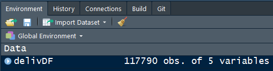 Figure 7.3: (ref:envData2
Notice that the environment tab has been updated (see Figure 7.3) to tell us that this is a data frame consisting of 117,790 observations and 5 variables. When we printed the tibble object to the console, the first 10 observations get printed and we see the class of the five columns. To the experienced eye, one notes that plannedShipDate and actualShipDate are character class objects (i.e. <chr>). As R novices, this is understandably overlooked, but it worth learning now that the class of an object determines what we can do with it. For example, the character class usually stores text information, also known as a string in computer lingo. As such, the following command trying to see the difference in planned versus ship dates for the first observation lacks meaning; afterall, what does it mean to subtract one word from another?:
## Error in delivDF$actualShipDate[1] - delivDF$plannedShipDate[1]: non-numeric
The resulting error suggests that R expects numbers to be subtracted; since text is not a number, there is no logical way to make this function work. So, we need another function to convert from character class to something that recognizes dates. And consistent with a theme we have been learning, we just need to find the right function; as usual the right function is in a package from the tidyverse. In this case, we use the ymd function from the lubridate package.
Getting R to agree that your data contains the dates and times you
think it does can be tricky. lubridate simplifies that.
Identify the order in which the year, month, and day appears in your
character vector of dates. Now arrange the letters y,
m, and d in the corresponding order. This
arrangement is the name of the function in lubridate that
will parse your dates. The dates in delivDF are given in
month-day-year order; hence the mdy function will convert
the column from character to date class. (See
(https://lubridate.tidyverse.org/) for more details.)
# Uncomment this line to install the lubridate package
# install.packages("lubridate")
library("lubridate")

# Create new data frame to represent cleaned data
shipDF = delivDF
shipDF$plannedShipDate = mdy(shipDF$plannedShipDate)
shipDF$actualShipDate = mdy(shipDF$actualShipDate)

# Print updated tibble
shipDF
## # A tibble: 117,790 × 5
## shipID plannedShipDate actualShipDate partID quantity
## <chr> <date> <date> <chr> <int>
## 1 10001 2013-11-06 2013-10-04 part92b16c5 6
## 2 10002 2013-10-15 2013-10-04 part66983b 2
## 3 10003 2013-10-25 2013-10-07 part8e36f25 1
## 4 10004 2013-10-14 2013-10-08 part30f5de0 1
## 5 10005 2013-10-14 2013-10-08 part9d64d35 6
## 6 10006 2013-10-14 2013-10-08 part6cd6167 15
## 7 10007 2013-10-14 2013-10-08 parta4d5fd1 2
## 8 10008 2013-10-14 2013-10-08 part08cadf5 1
## 9 10008 2013-10-14 2013-10-08 ship16 1
## 10 10008 2013-10-14 2013-10-08 ship22 1
## # ℹ 117,780 more rowsWith date classes in place, we can now take advantage of date arithmetic and lubridate functions. For example, how many days late was the first line item shipped?
## Time difference of -33 daysThe answer is it was not shipped late, it was actually shipped 33 days ahead of the planned ship date.
Other date operations include these:
## [1] "2025-01-15"## [1] 2025## [1] 1## [1] 15## [1] 4## [1] 15## [1] 15We can add a second argument, label = TRUE, to display the name of the weekday (represented as an ordered factor):
Notice that the wday function returns a
factor variable (i.e. its class is the factor
class). Factors are used to describe categorical variables with a fixed
and known set of levels. They are often tricky to deal with. For
historical context, see here: (https://tinyurl.com/y38wcekn).
## [1] Wed
## Levels: Sun < Mon < Tue < Wed < Thu < Fri < SatFor more date functions, see the RStudio “Dates and Times Cheat Sheet” ( (https://rstudio.github.io/cheatsheets/html/lubridate.html) ) and information about the lubridate package at the tidyverse website ( (https://lubridate.tidyverse.org/) ).
7.2 Lateness Calculation
Now that our data is loaded and cleaned, we want to determine whether a particular delivery of an order is late or not. Let’s revisit the data we have regarding deliveries:
## # A tibble: 117,790 × 5
##    shipID plannedShipDate actualShipDate partID      quantity
##    <chr>  <date>          <date>         <chr>          <int>
##  1 10001  2013-11-06      2013-10-04     part92b16c5        6
##  2 10002  2013-10-15      2013-10-04     part66983b         2
##  3 10003  2013-10-25      2013-10-07     part8e36f25        1
##  4 10004  2013-10-14      2013-10-08     part30f5de0        1
##  5 10005  2013-10-14      2013-10-08     part9d64d35        6
##  6 10006  2013-10-14      2013-10-08     part6cd6167       15
##  7 10007  2013-10-14      2013-10-08     parta4d5fd1        2
##  8 10008  2013-10-14      2013-10-08     part08cadf5        1
##  9 10008  2013-10-14      2013-10-08     ship16             1
## 10 10008  2013-10-14      2013-10-08     ship22             1
## # ℹ 117,780 more rowsand also revisit the CEO’s first question:
- Does service level (measured by on-time shipments) vary across product categories?
 Figure 7.4: Time to traverse the business analytics bridge.
It is time to cross the business analytics bridge (Figure 7.4). Notice that the data we have refers to shipments and parts. Notice that the CEO’s question talks about on-time shipments. We need to be mathematically precise in translating the CEO’s real-world concerns to mathematical calculations; did he really mean shipments, or perhaps orders, or maybe even partID’s? As an analyst, it is your job to form an opinion and validate that opinion with your stakeholder about how you plan to translate real-world concerns into mathematical constructs. Do not immediately fire off an email everytime you have a question; spend some time thinking and researching the issue before you make yourself look silly by asking simplistic questions that waste time. Also, when thinking about an issue, adopting the customer’s perspective is often a good starting point.
After deliberating, forming an opinion, and validating that opinion, here is what is discovered about measuring lateness at ZappTech:
- The lateness calculation would ideally look at customer orders (i.e.
orderID), but since we do not have that data and it is rare that an order gets broken into mulitple shipments, usingshipIDas the observational unit should give a good estimate/proxy of on-time order performance. - Measuring lateness using quantity does not make sense for ZappTech. Some products, like latex gloves, get ordered by the hundreds whereas machines get ordered one or two at a time.
- Measuring lateness by
partIDmight make sense for evaluating inventory policies on specific parts, but for now talking about lateness byshipIDis preferable. - For each unique shipID, if
actualShipDate > plannedShipDate, then the shipID is considered late. (Note: it has been verified that each shipID has one and only one actualShipDate).
With these assumptions about measuring lateness, we can now rigorously define what it means to be late in mathematical and computational terms.
7.2.1 Using dplyr to compute lateness
Each line in shipDF represents a unique shipID/partID combination. Since the partID information is unnecessary, we create a new data frame to isolate just the shipment information:
# load dpyr package for select() and distinct()
library("dplyr")

# create new data frame for just shipID date info
shipDateDF = shipDF %>%
  select(shipID,plannedShipDate,actualShipDate) %>%
  distinct()  ## get unique rows
              ## to avoid double-counting

shipDateDF
## # A tibble: 23,339 × 3
## shipID plannedShipDate actualShipDate
## <chr> <date> <date>
## 1 10001 2013-11-06 2013-10-04
## 2 10002 2013-10-15 2013-10-04
## 3 10003 2013-10-25 2013-10-07
## 4 10004 2013-10-14 2013-10-08
## 5 10005 2013-10-14 2013-10-08
## 6 10006 2013-10-14 2013-10-08
## 7 10007 2013-10-14 2013-10-08
## 8 10008 2013-10-14 2013-10-08
## 9 10009 2013-10-14 2013-10-08
## 10 10010 2013-10-14 2013-10-08
## # ℹ 23,329 more rowsifelse() is a function from base R (i.e. no need to load
a package). The function tests a logical condition in its first
argument. If the test is TRUE, ifelse()
returns the second argument. If the test is FALSE,
ifelse() returns the third argument. The function is
vectorized - it takes a vector as input and outputs a vector. In
contrast, an aggregate function (like sum()) will take a
vector of input and output a scalar (i.e. a single element). For more on
vectorized functions, see Noam
Ross’s Vectorization in R: Why?.
Now, add a column to capture lateness.
shipDateDF = shipDateDF %>%
  mutate(lateFlag =
           ifelse(actualShipDate > plannedShipDate,
                  TRUE,
                  FALSE))

shipDateDF
## # A tibble: 23,339 × 4
## shipID plannedShipDate actualShipDate lateFlag
## <chr> <date> <date> <lgl>
## 1 10001 2013-11-06 2013-10-04 FALSE
## 2 10002 2013-10-15 2013-10-04 FALSE
## 3 10003 2013-10-25 2013-10-07 FALSE
## 4 10004 2013-10-14 2013-10-08 FALSE
## 5 10005 2013-10-14 2013-10-08 FALSE
## 6 10006 2013-10-14 2013-10-08 FALSE
## 7 10007 2013-10-14 2013-10-08 FALSE
## 8 10008 2013-10-14 2013-10-08 FALSE
## 9 10009 2013-10-14 2013-10-08 FALSE
## 10 10010 2013-10-14 2013-10-08 FALSE
## # ℹ 23,329 more rowsAnd now, we take advantage of the fact that R treats logical (TRUE/FALSE) values as numbers when used with numeric functions. TRUE is converted to 1 and FALSE converted to 0. Thus, as a simple example of this, we have:
# make a vector of 2 - TRUE values and 3 FALSE values
logicalVector = c(TRUE,TRUE,FALSE,FALSE,FALSE)

## return # of TRUE values
sum(logicalVector)
## [1] 2## [1] 0.4## [1] 1 1 0 0 0For calculating late shipments, the following code collapses the data on 23,339 shipments into two rows: one for on-time shipments (i.e. lateFlag = FALSE) and one for late shipments (i.e. lateFlag = TRUE):
shipDateDF %>%
  group_by(lateFlag) %>%
  summarize(countLate = n()) %>%
  mutate(proportion = countLate / sum(countLate))
## # A tibble: 2 × 3
## lateFlag countLate proportion
## <lgl> <int> <dbl>
## 1 FALSE 21399 0.917
## 2 TRUE 1940 0.0831** To calculate the new proportion column, the 2-element
countLate vector (i.e. 21399,1940) is divided by the
aggregated 1-element sum(countLate) vector
(i.e. 21399+1940). In R, when two unequal length vectors are
arithmetically combined, the shorter vector is recycled so that it has
the same length as the longer vector. Thus,
c(1,2,3) + c(4,5) = c(1+4,2+5,3+4) = c(5,7,7). See
(https://r4ds.hadley.nz/numbers#sec-recycling) for more info. And in
this case, we get two elements returned (i.e. 21399 / (21399+1940) ,
1940 / (21399+1940)).
where the last mutate seems almost magical, but amazingly works.\(^{**}\) We now have a lateness calculation complete, 8.31% of shipments are being delivered later than planned.
7.3 Bringing in Product Category Information
The information contained in shipDF does not include product category information. This information happens to be in another table:
## # A tibble: 12,026 × 3
##    partID      productLine prodCategory
##    <chr>       <chr>       <chr>
##  1 part0a7f7c6 line7a      Machines
##  2 part84778b6 line7a      Machines
##  3 part330b1c9 line6d      Machines
##  4 parta4ebc9b line6d      Machines
##  5 partcf299b0 line6d      Machines
##  6 partfbc80a  line6d      Machines
##  7 partc986d3f line6d      Machines
##  8 part38c7896 line6d      Machines
##  9 partc39b72f line6d      Machines
## 10 partd8ab54  line6d      Machines
## # ℹ 12,016 more rows
So now, we want to calculate lateness by product category, but the product category information is in prodLineDF and the actual/planned shipment data is in shipDF. How might we combine the information from these two tables?
In dplyr, there are many ways to integrate two data frames, we will focus on the one we need, called a left join. For the moment, let’s ignore our need to combine shipping data with product category information and just learn about how a left join works.
7.3.1 The left_join() Function
For more information on methods of joining data frames, see (https://r4ds.hadley.nz/joins),
The left_join() function includes all observations from one data frame and appends matching columns from another data frame. This is a commonly used join because it ensures you don’t lose observations from your primary data frame. Let’s see this in action using two simple data frames; one contains job title information and the other contains hourly salary:
employeeDF = tibble(
  name = c("Adam","Bob","Charlie"),
  title = c("Server I","Innkeeper III","Server II"))

employeeDF
## # A tibble: 3 × 2
## name title
## <chr> <chr>
## 1 Adam Server I
## 2 Bob Innkeeper III
## 3 Charlie Server IIsalaryDF = tibble( ## left parantheses
title = c("Server I","Server II",
"Server III","Innkeeper I",
"Innkeeper II","Innkeeper III",
"Bartender I","Bartender II"),
hourlySalary = c(11,14,17,21,26,32,12,13)
) ## right parantheses
salaryDF## # A tibble: 8 × 2
## title hourlySalary
## <chr> <dbl>
## 1 Server I 11
## 2 Server II 14
## 3 Server III 17
## 4 Innkeeper I 21
## 5 Innkeeper II 26
## 6 Innkeeper III 32
## 7 Bartender I 12
## 8 Bartender II 13Given these two tables, we can find the hourly salary for each of the three employees using left_join(), a dplyr function. One could write left_join(employeeDF,salaryDF), but with experience you will find it more elegant and intuitive to use the chaining operator from dplyr as shown:
## # A tibble: 3 × 3
##   name    title         hourlySalary
##   <chr>   <chr>                <dbl>
## 1 Adam    Server I                11
## 2 Bob     Innkeeper III           32
## 3 Charlie Server II               14
Behind the scenes, dplyr() knows to combine the data frames based on any commonly labeled column names. In the above example, this was the title column; for all records in employeeDF append the columns of salaryDF by using the title column for matching rows of the data frames. Arguments to the left_join() function can be used to further control this behavor (see (https://r4ds.hadley.nz/joins)).
7.3.2 Combining Shipment Data With Product Category Data
Having learned to do a left_join(), we are equipped to get product category information and shipment information into one data frame. The first data frame, the primary one, will be shipment information since we want to know about shipped partID’s, not necessarily all the partID’s in prodLineDF.
You may notice that some of the product category information is
listed as NA. In R, missing values are represented by the
symbol NA (not available) . Impossible values (e.g., dividing by zero)
are represented by the symbol NaN (not a number). In this
case, these NA’s do have meaning though. Specifically,
these are partID’s in the original data that we do not know
the product category for. To the left, we filter out these rows. In the
real-world, verify that this filtering makes sense for your data.
catDF = shipDF %>%
  left_join(prodLineDF) %>%
  # NA prodCategory are for partID's that are
  # not really parts.  Used for shipping or
  # service fees, so we can safely get rid of them
  filter(!is.na(prodCategory))

catDF
## # A tibble: 98,207 × 7
## shipID plannedShipDate actualShipDate partID quantity productLine prodCategory
## <chr> <date> <date> <chr> <int> <chr> <chr>
## 1 10001 2013-11-06 2013-10-04 part92b16c5 6 line4b Machines
## 2 10002 2013-10-15 2013-10-04 part66983b 2 linea3 Marketables
## 3 10003 2013-10-25 2013-10-07 part8e36f25 1 line90 Machines
## 4 10004 2013-10-14 2013-10-08 part30f5de0 1 linea3 Marketables
## 5 10005 2013-10-14 2013-10-08 part9d64d35 6 line9b Machines
## 6 10006 2013-10-14 2013-10-08 part6cd6167 15 linec1 Marketables
## 7 10007 2013-10-14 2013-10-08 parta4d5fd1 2 line55 SpareParts
## 8 10008 2013-10-14 2013-10-08 part08cadf5 1 line4b Machines
## 9 10009 2013-10-14 2013-10-08 part5cc4989 10 linec1 Marketables
## 10 10010 2013-10-14 2013-10-08 part912ae4c 1 line4b Machines
## # ℹ 98,197 more rows7.4 Answering the CEO’s Questions
With all the data we need to answer questions in one data frame, we proceed.
7.4.1 Does service level (measured by on-time shipments) vary across product categories?
catDF %>%
  select(shipID,
         plannedShipDate,
         actualShipDate,
         prodCategory) %>%
  distinct() %>% ## one row per shipment/prodCategory
  mutate(lateFlag =
           ifelse(actualShipDate > plannedShipDate,
                  TRUE,
                  FALSE)) %>%
  group_by(prodCategory,lateFlag) %>%
  summarize(countLate = n()) %>%
  mutate(proportion = countLate / sum(countLate)) %>%
  arrange(lateFlag,proportion)
## # A tibble: 8 × 4
## # Groups: prodCategory [4]
## prodCategory lateFlag countLate proportion
## <chr> <lgl> <int> <dbl>
## 1 Machines FALSE 3124 0.810
## 2 SpareParts FALSE 4561 0.842
## 3 Liquids FALSE 6512 0.919
## 4 Marketables FALSE 13910 0.919
## 5 Marketables TRUE 1222 0.0808
## 6 Liquids TRUE 575 0.0811
## 7 SpareParts TRUE 857 0.158
## 8 Machines TRUE 732 0.190From the above analysis, we find that there does seem to be discrepancies between on-time shipments by product category. Machines has the most late shipments (19%), SpareParts(15.8%) is next, and the remaining two, Liquids (8.1%) and Marketables (8.1%) have similar performance.
7.4.2 How often do orders include products from more than one product category?
Now, we answer how often do orders (i.e. shipments) include products from other product categories using group_by() and summarize()?
With these large code blocks of simple verbs chained together, take
your time to figure out each step. For example, I might first run
catDF, then catDF %>% select(shipID,\(\cdots\)), then
catDF %>% select(shipID,\(\cdots\)) %>% distinct().
Only after continuing this pattern for each step in the chain would I
worry about creating the numCatDF object created in the
code to the left.
# find # of categories included on each shipID
numCatDF = catDF %>%
  select(shipID,
         plannedShipDate,
         actualShipDate,
         prodCategory) %>%
  distinct() %>% # unique rows only
  group_by(shipID) %>%
  summarize(numCategories = n())

# print out summary of numCategories column
numCatDF %>%
  group_by(numCategories) %>%
  summarize(numShipID = n()) %>%
  mutate(percentOfShipments =
           numShipID / sum(numShipID))
## # A tibble: 4 × 3
## numCategories numShipID percentOfShipments
## <int> <int> <dbl>
## 1 1 17993 0.775
## 2 2 3261 0.141
## 3 3 842 0.0363
## 4 4 1113 0.0480The answer to this second question is about 22.5% of orders contain more than one product category. So, in conclusion, 22.5% of orders have more than one product category on them and yes, it does seem that the product categories are managed differently.
Recommendation to the CEO: Product categories do have different performance characteristics in regards to late shipments: Machines(19%), SpareParts(15.8%), Liquids (8.1%), and Marketables (8.1%). And yes, consumers often buy from multiple categories (22.5%). So service levels do differ by category, but it is unknown whether this is an issue for consumers. Hire our team again and we can dig deeper into whether customer behavior changes as result of late shipments from a particular product category.
7.5 Notes About Data Wrangling from Twitter
Data cleaning/wrangling/munging is the process of transforming raw data into a more valuable and useful format. In real-world data analysis, much of your time will be spent doing this. While consuming this textbook, much of the data will be presented in a format that is amenable for analysis; the real-world is much less thoughtful in this regard. Please see this collection of tweets (Figure 7.5) to give you an idea about real-world data wrangling:
Figure 7.5: Some insightful tweets about data cleaning/wrangling.


Do not be surprised or think that you are wasting time when data wrangling. This is a necessary - albeit frustrating at times - part of the BAW.
7.6 Getting Help
For dealing with factors, see McNamara and Horton (2018McNamara, Amelia, and Nicholas J Horton. 2018. “Wrangling Categorical Data in r.” The American Statistician 72 (1): 97–104.). For more notes on logical vectors see (https://bookdown.org/ndphillips/YaRrr/logical-indexing.html).
7.7 Exercises
For all the exercises, be sure to use the chaining operator and also, download data from a github repository that I maintain. The data gives US county demographic information in 2016 as well as a snapshot of some primary voting data in the United States. Here is the code to get this data into two dataframes called countyDF and primaryDF:
library(tidyverse)
countyDF = readr::read_csv(
  file = "https://raw.githubusercontent.com/flyaflya/persuasive/main/county_facts.csv",
  show_col_types = FALSE)
primaryDF = readr::read_csv(
  file = "https://raw.githubusercontent.com/flyaflya/persuasive/main/primary_results.csv",
  show_col_types = FALSE)
Exercise 7.1 How many votes has the leading Democrat presidential candidate accumulated?
Exercise 7.2 How many votes has the leading Republican presidential candidate accumulated?
Exercise 7.3 Which county (areaName) had the largest number of voters for Republican candidates? (hint: if you want to usearrange after a group_by, use ungroup() so the ordering is for the entire dataframe and not just ordered within groups)
Exercise 7.4 Which state (stateAbbrev) had the county (areaName) where 81,931 voters turned out for the Republican primary? (hint: if you want to usearrange after a group_by, use ungroup() so the ordering is for the entire dataframe and not just ordered within groups)
Exercise 7.5 What percentage of the republican vote in Iowa did Ben Carson receive among counties where the median income is greater than $50,000 (enter as decimal to the nearest thousandth place, for example, 0.062, 0.124, etc)?
Exercise 7.6 For this question, assume that there is no distinction between Republicans and Democrats; all votes cast count equally. Calculate the percentage of all votes (Democrat + Republican) placed in each county that each candidate received. For the county where Hillary Clinton achieved her largest percentage of votes, what percentage of the vote did she earn (report as a decimal to the nearest thousandth place, for example, 0.062, 0.124, etc)?
Exercise 7.7 For this question, assume that there is no distinction between Republicans and Democrats; all votes cast count equally. Calculate the percentage of all votes (Democrat + Republican) placed in each county that each candidate received. For the county where Ted Cruz achieved his largest percentage of votes, what percentage of the vote did he earn (report as a decimal to the nearest thousandth place, for example, 0.062, 0.124, etc)?