Chapter 6 dplyr: Manipulating Data Frames
To work with data, we need a place to store it in R. Our default setting is to store data in data frames in a format amenable to analysis\(^{**}\). When we work with data frames, \(^{**}\) Data will not always be stored in a way that is amenable to analysis. Typically, we will get our data into a tidy format - such that each row represents an observation and each column represents an attribute or property of that observation think of each data frame as a collection of observations with each observation in its own row and each recorded variable (e.g. measurement) represented in a column; a generic dataframe with \(M\) rows and \(N+1\) columns (i.e. \(N\) variables plus an id column) is shown in Table 6.1.
Table 6.1: Think of a data frame as consisting of rows of observations and columns of variables.
| observationID | var1 | var2 | var… | varN |
|---|---|---|---|---|
| 1 | xx | xx | xx | xx |
| 2 | xx | xx | xx | xx |
| \(\vdots\) | \(\vdots\) | \(\vdots\) | \(\vdots\) | \(\vdots\) |
| M | xx | xx | xx | xx |
We can look at a subset of the built-in mtcars dataset as a more tangible example of a dataframe - from the console, type mtcars and press <ENTER>:
| carID | mpg | cyl | disp | hp | drat | wt | qsec | vs | am | gear | carb |
|---|---|---|---|---|---|---|---|---|---|---|---|
| Mazda RX4 | 21.0 | 6 | 160.0 | 110 | 3.90 | 2.620 | 16.46 | 0 | 1 | 4 | 4 |
| Honda Civic | 30.4 | 4 | 75.7 | 52 | 4.93 | 1.615 | 18.52 | 1 | 1 | 4 | 2 |
| Camaro Z28 | 13.3 | 8 | 350.0 | 245 | 3.73 | 3.840 | 15.41 | 0 | 0 | 3 | 4 |
| Volvo 142E | 21.4 | 4 | 121.0 | 109 | 4.11 | 2.780 | 18.60 | 1 | 1 | 4 | 2 |
Each row represents a particular car and the recorded data associated with each car is organized by column. Note that an ID column is also just an attribute of that observation. This is a format that we can easily digest. Another format, which we will call a long dataframe, might look like this:
| carID | measure | value |
|---|---|---|
| Mazda RX4 | mpg | 21.0 |
| Honda Civic | mpg | 30.4 |
| Camaro Z28 | mpg | 13.3 |
| Volvo 142E | mpg | 21.4 |
| Mazda RX4 | cyl | 6.0 |
| Honda Civic | cyl | 4.0 |
| Camaro Z28 | cyl | 8.0 |
| Volvo 142E | cyl | 4.0 |
where the observational unit can be thought of as a measurement (e.g. mpg for a Mazda RX4), but a single car’s various measurements span multiple rows. This longer format, sometimes considered a tidy format, is often useful for plotting.
There are infinite ways data can be made harder to work with. Here, is just one example:
| carID | mpg | eng:cyl_disp | hp | drat | wt | qsec | vs | am | gear | carb |
|---|---|---|---|---|---|---|---|---|---|---|
| Mazda RX4 | 21.0 | 6 - 160 | 110 | 3.90 | 2.620 | 16.46 | 0 | 1 | 4 | 4 |
| Honda Civic | 30.4 | 4 - 75.7 | 52 | 4.93 | 1.615 | 18.52 | 1 | 1 | 4 | 2 |
| Camaro Z28 | 13.3 | 8 - 350 | 245 | 3.73 | 3.840 | 15.41 | 0 | 0 | 3 | 4 |
| Volvo 142E | 21.4 | 4 - 121 | 109 | 4.11 | 2.780 | 18.60 | 1 | 1 | 4 | 2 |
where multiple variables (i.e. cyl and disp) might be stored together in one column. See (https://tidyr.tidyverse.org/articles/tidy-data.html) for further examples of messy data and a discussion of tidy data principles.
6.1 Tibbles
While R’s data frame object has been the long running standard placeholder for data, we will often convert data frame’s into tibble objects. The as_tibble function from the dplyr package does this conversion for us:
Remember, in order to load a package into an R session using
library(packageName), you must have the package installed
on your system. dplyr was installed in previous chapters,
so this code should work without error.
# make the dplyr package and its function available
# in the current R session.
library(dplyr)

## convert the built in mtcars dataframe to a tibble
as_tibble(mtcars)
## # A tibble: 32 × 11
## mpg cyl disp hp drat wt qsec vs am gear carb
## <dbl> <dbl> <dbl> <dbl> <dbl> <dbl> <dbl> <dbl> <dbl> <dbl> <dbl>
## 1 21 6 160 110 3.9 2.62 16.5 0 1 4 4
## 2 21 6 160 110 3.9 2.88 17.0 0 1 4 4
## 3 22.8 4 108 93 3.85 2.32 18.6 1 1 4 1
## 4 21.4 6 258 110 3.08 3.22 19.4 1 0 3 1
## 5 18.7 8 360 175 3.15 3.44 17.0 0 0 3 2
## 6 18.1 6 225 105 2.76 3.46 20.2 1 0 3 1
## 7 14.3 8 360 245 3.21 3.57 15.8 0 0 3 4
## 8 24.4 4 147. 62 3.69 3.19 20 1 0 4 2
## 9 22.8 4 141. 95 3.92 3.15 22.9 1 0 4 2
## 10 19.2 6 168. 123 3.92 3.44 18.3 1 0 4 4
## # ℹ 22 more rowsThe main advantage of a tibble is that when it is printed out, it will not try to print all the data. By default, tibble’s show the first 10 rows of data and as many columns as will fit on your screen. Once we start working with datasets that have tens of thousands of rows and dozens of columns, you will then appreciate the tibble. In this book, we will use the terms tibble and data frame synonymously because they differ only very slightly in their behavior. Most of the time, Internet resources will almost exclusively refer to data frames as the object for data storage - the tibble terminology is far less ubiquitous - so use data frame as your google search term.
6.2 Reducing Cognitive Load
 Figure 6.1: What time does this clock read? A non-standardized design increases the amount of thinking time required to get the answer. After significant deliberation, hopefully you see that the time is 7:11.
Data manipulation is not a natural human task - there is definitely some mental gymnastics required. To simplify the cognitive load, we will adopt a standard way of thinking about data manipulation. These standards will reduce the cognitive load, i.e. thinking time, required of your brain as you get data into more useful forms. An example standard that you might take for granted is that used by clock makers; see the example in Figure 6.1 and you will quickly realize, by example, how important standards can be in aiding your thinking (example from Norman 2013Norman, Don. 2013. The Design of Everyday Things: Revised and Expanded Edition. Basic Books (AZ).).
When it comes to data manipulation, the standards we will learn in this chapter are implemented in the dplyr package. The dplyr package is part of the tidyverse (https://www.tidyverse.org/) ecosystem of packages. These packages are all designed to reduce cognitive load through a set of well-thought out standards which share an underlying design philosophy and structure. The dplyr package simplifies our thought process in regards to data manipulation by reducing our possible operations to five main verbs and one adverb. It then facilitates the chaining of these operations to accomplish even the most difficult of data manipulation tasks. The five main verbs are:
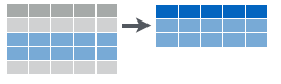 Figure 6.2: Filtering data to get a subset of rows.
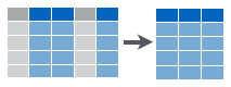 Figure 6.3: Selecting data to get a subset of columns.
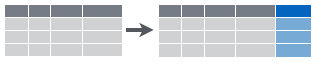 Figure 6.4: Create new columns that are functions of existing columns using mutate.
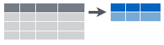 Figure 6.5: Collapsing data into summary metrics using summarize.
filter(): select subset of rows (i.e. observations). See Figure 6.2.arrange(): reorder rowsselect(): select subset of columns (i.e. variables). See Figure 6.3.mutate(): create new columns that are functions of existing columns. See Figure 6.4.summarize(): collapse data into a single row. See Figure 6.5.
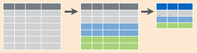 Figure 6.6: Collapsing data into summary metrics using
 group_by() with summarize().
These verbs are useful on their own, but they become really powerful when you apply them to groups of observations within a dataset using the group_by() function (i.e. the one adverb). It breaks down a dataset into specified groups of rows so that subsequent verbs may act on grouped rows and not just the entire dataset.
Grouping affects the verbs as follows:
arrange()orders first by the grouping variables and then by the variables of arrangesummarize()is the most powerful to combine with grouping. You usesummarizewith aggregate functions, which take a vector of values and return a single number. See Figure 6.6. There are many useful examples of aggregate functions in base R likemin(),max(),mean(),sum(),sd(),median(), andIQR().dplyrprovides a handful of others:n(): the number of observations in the current groupn_distinct(): the number of unique values in x.first(x), last(x)andnth(x, n): these work similarly tox[1],x[length(x)], andx[n], but give you more control over the result if the value is missing.
Learning dplyr is perhaps easiest by example. Below, we will provide code for you to follow the vignette that accompanies the dplyr package.\(^{**}\) see https://dplyr.tidyverse.org/ if interested in more detail We’ll start with the built in nycflights13 data frame. This dataset contains all 336,776 flights that departed from New York City in 2013 (see link in margin).
## Uncomment the install line if the package has not
## been installed on your computer.
#install.packages("nycflights13", dependencies = TRUE)
#install.packages("dplyr", dependencies = TRUE)
library(nycflights13)
library(dplyr)

## Show the dataframe in the RStudio envirnoment
flights = flights

## just fyi, there are lots of datasets already in R
data()
6.3 filter() Rows
filter allows you to select a subset of rows in a data frame. The first argument is the name of the data frame. The second and subsequent arguments are the expressions that filter the data frame:
For example, we can select all flights on January 1st with:Take note of the double equal sign \(==\) which is used for logical comparison. The single equal sign \(=\) is only used for assignment purposes.
## # A tibble: 842 × 19
##     year month   day dep_time sched_dep_time dep_delay arr_time sched_arr_time
##    <int> <int> <int>    <int>          <int>     <dbl>    <int>          <int>
##  1  2013     1     1      517            515         2      830            819
##  2  2013     1     1      533            529         4      850            830
##  3  2013     1     1      542            540         2      923            850
##  4  2013     1     1      544            545        -1     1004           1022
##  5  2013     1     1      554            600        -6      812            837
##  6  2013     1     1      554            558        -4      740            728
##  7  2013     1     1      555            600        -5      913            854
##  8  2013     1     1      557            600        -3      709            723
##  9  2013     1     1      557            600        -3      838            846
## 10  2013     1     1      558            600        -2      753            745
## # ℹ 832 more rows
## # ℹ 11 more variables: arr_delay <dbl>, carrier <chr>, flight <int>,
## #   tailnum <chr>, origin <chr>, dest <chr>, air_time <dbl>, distance <dbl>,
## #   hour <dbl>, minute <dbl>, time_hour <dttm>
6.4 arrange() Rows
arrange() works similarly to filter() except that instead of filtering or selecting rows, it reorders them. It takes a data frame, and a set of column names (or more complicated expressions) to order by. If you provide more than one column name, each additional column will be used to break ties in the values of preceding columns.
## # A tibble: 336,776 × 19
##     year month   day dep_time sched_dep_time dep_delay arr_time sched_arr_time
##    <int> <int> <int>    <int>          <int>     <dbl>    <int>          <int>
##  1  2013     1     1      517            515         2      830            819
##  2  2013     1     1      533            529         4      850            830
##  3  2013     1     1      542            540         2      923            850
##  4  2013     1     1      544            545        -1     1004           1022
##  5  2013     1     1      554            600        -6      812            837
##  6  2013     1     1      554            558        -4      740            728
##  7  2013     1     1      555            600        -5      913            854
##  8  2013     1     1      557            600        -3      709            723
##  9  2013     1     1      557            600        -3      838            846
## 10  2013     1     1      558            600        -2      753            745
## # ℹ 336,766 more rows
## # ℹ 11 more variables: arr_delay <dbl>, carrier <chr>, flight <int>,
## #   tailnum <chr>, origin <chr>, dest <chr>, air_time <dbl>, distance <dbl>,
## #   hour <dbl>, minute <dbl>, time_hour <dttm>
Use desc() to order a column in descending order
## # A tibble: 336,776 × 19
##     year month   day dep_time sched_dep_time dep_delay arr_time sched_arr_time
##    <int> <int> <int>    <int>          <int>     <dbl>    <int>          <int>
##  1  2013     1     9      641            900      1301     1242           1530
##  2  2013     6    15     1432           1935      1137     1607           2120
##  3  2013     1    10     1121           1635      1126     1239           1810
##  4  2013     9    20     1139           1845      1014     1457           2210
##  5  2013     7    22      845           1600      1005     1044           1815
##  6  2013     4    10     1100           1900       960     1342           2211
##  7  2013     3    17     2321            810       911      135           1020
##  8  2013     7    22     2257            759       898      121           1026
##  9  2013    12     5      756           1700       896     1058           2020
## 10  2013     5     3     1133           2055       878     1250           2215
## # ℹ 336,766 more rows
## # ℹ 11 more variables: arr_delay <dbl>, carrier <chr>, flight <int>,
## #   tailnum <chr>, origin <chr>, dest <chr>, air_time <dbl>, distance <dbl>,
## #   hour <dbl>, minute <dbl>, time_hour <dttm>
6.5 select() Columns
Often you work with large datasets with many columns, but only a few are actually of interest to you. select() allows you to rapidly zoom in on a useful subset of columns:
## # A tibble: 336,776 × 3
##     year month   day
##    <int> <int> <int>
##  1  2013     1     1
##  2  2013     1     1
##  3  2013     1     1
##  4  2013     1     1
##  5  2013     1     1
##  6  2013     1     1
##  7  2013     1     1
##  8  2013     1     1
##  9  2013     1     1
## 10  2013     1     1
## # ℹ 336,766 more rows## # A tibble: 336,776 × 3
## year month day
## <int> <int> <int>
## 1 2013 1 1
## 2 2013 1 1
## 3 2013 1 1
## 4 2013 1 1
## 5 2013 1 1
## 6 2013 1 1
## 7 2013 1 1
## 8 2013 1 1
## 9 2013 1 1
## 10 2013 1 1
## # ℹ 336,766 more rows## # A tibble: 336,776 × 16
## dep_time sched_dep_time dep_delay arr_time sched_arr_time arr_delay carrier
## <int> <int> <dbl> <int> <int> <dbl> <chr>
## 1 517 515 2 830 819 11 UA
## 2 533 529 4 850 830 20 UA
## 3 542 540 2 923 850 33 AA
## 4 544 545 -1 1004 1022 -18 B6
## 5 554 600 -6 812 837 -25 DL
## 6 554 558 -4 740 728 12 UA
## 7 555 600 -5 913 854 19 B6
## 8 557 600 -3 709 723 -14 EV
## 9 557 600 -3 838 846 -8 B6
## 10 558 600 -2 753 745 8 AA
## # ℹ 336,766 more rows
## # ℹ 9 more variables: flight <int>, tailnum <chr>, origin <chr>, dest <chr>,
## # air_time <dbl>, distance <dbl>, hour <dbl>, minute <dbl>, time_hour <dttm>A common use of select() is to pair it with the distinct() verb (a shortcut variant for the filter() verb). This combination returns the unique rows of a smaller data frame. Here we use select() to get just one column (tailNum) and then distinct() returns the unique tail numbers of all the airplanes in the dataset:
## # A tibble: 4,044 × 1
##    tailnum
##    <chr>
##  1 N14228
##  2 N24211
##  3 N619AA
##  4 N804JB
##  5 N668DN
##  6 N39463
##  7 N516JB
##  8 N829AS
##  9 N593JB
## 10 N3ALAA
## # ℹ 4,034 more rows
6.6 Add New Columns with Mutate()
Besides selecting sets of existing columns, it’s often useful to add new columns that are functions of existing columns. This is the job of mutate():
flightSpeedDF = select(flights, distance, air_time)
mutate(flightSpeedDF,
  speed = distance / air_time * 60)
## # A tibble: 336,776 × 3
## distance air_time speed
## <dbl> <dbl> <dbl>
## 1 1400 227 370.
## 2 1416 227 374.
## 3 1089 160 408.
## 4 1576 183 517.
## 5 762 116 394.
## 6 719 150 288.
## 7 1065 158 404.
## 8 229 53 259.
## 9 944 140 405.
## 10 733 138 319.
## # ℹ 336,766 more rowsThe second argument to the mutate() function (e.g. speed = distance / air_time * 60) defines a new column called speed and it is a function of the existing columns distance and air.
6.7 summarize() Values
The last verb is summarize(). It collapses a data frame into a single row by aggregating a column of data. Below, the dep_delay column is summarized using the mean() function:
## # A tibble: 1 × 1
##   delay
##   <dbl>
## 1  12.6
So instead of seeing a data frame with 336,776 rows, we collapse all those departure delays into a single average number (i.e. 12.6 minutes).
6.8 Grouped Operations with group_by()
These five functions provide the basis of our data manipulation language. At the most basic level, you can only alter a data frame in five useful ways: you can reorder the rows (arrange()), filter the rows (filter()), pick columns of interest (select()), add new columns (mutate()) that are functions of existing variables, or collapse (summarize()) many rows into a summary. The power of the language comes from your ability to combine the five functions, but before we do that - let’s discuss one more function group_by().
The group_by() function does not change the output of a data frame. But it does change how arrange(), mutate(), and summarize() behave. Each of them will act within the unique values of specified grouping variable(s) as if the rows of the data frame were separated into groups before the other verb is called. This is easiest to see by example via the powerful data manipulation enabled by combining group_by() and summarize() functions. The summarize operation will collapse each group of data instead of the entire dataset into a single row. For example, we could use these to find the number of planes and the number of flights that go to each possible destination:
## create a new dataframe that is organized by groups
destinations = group_by(flights, dest)
## summarize the rows of the grouped data frame
destDF = summarize(destinations,
  planes = n_distinct(tailnum), # unique planes
  flights = n() # number of flights
)
destDF
## # A tibble: 105 × 3
## dest planes flights
## <chr> <int> <int>
## 1 ABQ 108 254
## 2 ACK 58 265
## 3 ALB 172 439
## 4 ANC 6 8
## 5 ATL 1180 17215
## 6 AUS 993 2439
## 7 AVL 159 275
## 8 BDL 186 443
## 9 BGR 46 375
## 10 BHM 45 297
## # ℹ 95 more rows6.9 Commonalities
You may have noticed that the function syntax for all these verbs is very similar:
- The first argument is a data frame (e.g.
flightsorflightsDF). - The subsequent arguments describe what to do with the data frame. Notice that you can refer to columns in the data frame directly without using $. Hence, you do NOT have to write something like
flights$dep_delayin the abovesummarize()function. - The resulting output is a new data frame.
As is shown in the next section, these properties make it easy to chain together multiple simple steps to achieve a complex result.
6.10 Chaining with %>%
In the previous examples, we sometimes had to save results to intermediate dataframes and then do subsequent analysis on the newly created dataframe. For example, if using the original flights data frame we wanted to find the destination airports that had the fastest average (mean) flight speed, we could do the following:
# create new data frame (df) with three columns
# extracted from flights data frame
lightSpeedDF = select(flights, distance, air_time, dest)
# create new data frame with additional column
# representing speed
lightSpeedDF2 = mutate(lightSpeedDF,
                       speed = distance / air_time * 60)
# create new data frame that has hidden groupings
# by destination
lightSpeedDF3 = group_by(lightSpeedDF2, dest)
# create new data frame that summarizes speed for
# each destination group
lightSpeedDF4 = summarize(
  lightSpeedDF3,
  avgSpeed = mean(speed, na.rm = TRUE))
# print out a sorted data frame - note that the
# below does not create a new data frame
# as there is no assignment operator (i.e. '=')
arrange(lightSpeedDF4, desc(avgSpeed))
## # A tibble: 105 × 2
## dest avgSpeed
## <chr> <dbl>
## 1 ANC 490.
## 2 BQN 487.
## 3 SJU 486.
## 4 HNL 484.
## 5 PSE 481.
## 6 STT 479.
## 7 LAX 453.
## 8 SAN 451.
## 9 SMF 451.
## 10 LGB 450.
## # ℹ 95 more rowsAs an example of the chaining operator in mathematical notation,
assume \(f(x,y) = 2*x + y^2\). Then,
\(f(1,3) = 2*1 + 3^2 = 11\). To write
this with chaining, we have \(1\)
%>% \(f(3)\). Notice
that \(3\) %>% \(f(1)\) yields different results; in this
case, \(3\) %>% \(f(1) = f(3,1) = 7\).
This becomes challenging code. It creates several data frames that we are not interested in (e.g. lightSpeedDF2) and is difficult to read. Alternatively, we can leverage the chaining operator, %>%. This operator inserts an R object as the first argument of a function. In mathematical terms, \(x\) %>% \(f(y)\) is interpreted as \(f(x,y)\) - the \(x\) gets inserted as the first argument of the function. In other words, instead of continually writing functions of the form:
We can now go directly to the data frame we want:
without all of the intermediate data frames being created.
To find the fastest average flight speed destination:
flights %>%
select(distance, air_time, dest) %>%
mutate(speed = distance / air_time * 60) %>%
group_by(dest) %>%
summarize(avgSpeed = mean(speed, na.rm = TRUE)) %>%
arrange(desc(avgSpeed))and we can see this is much more succinct than the original method without chaining:
## # A tibble: 105 × 2
##    dest  avgSpeed
##    <chr>    <dbl>
##  1 ANC       490.
##  2 BQN       487.
##  3 SJU       486.
##  4 HNL       484.
##  5 PSE       481.
##  6 STT       479.
##  7 LAX       453.
##  8 SAN       451.
##  9 SMF       451.
## 10 LGB       450.
## # ℹ 95 more rows6.11 Cheatsheets And Some Variants of The Five Verbs
Tip: Print out the Data Transormation Cheat Sheet and place the pages on the wall behind your computer: https://github.com/rstudio/cheatsheets/raw/master/data-transformation.pdf
RStudio has done a wonderful job consolidating the most useful dplyr workflows into a two-page cheatsheet (see the “Data Transformation Cheat Sheet” at (https://posit.co/resources/cheatsheets/) ). While for teaching purposes, there are five main verbs and one helper verb (i.e. group_by()), the cheat sheet reveals that there are some variants of those verbs; these provide shortcuts to common workflows. A table of commonly used variants is given here:
| Primary Verb | Variant | Variant Description |
|---|---|---|
filter() |
distinct() |
Remove all duplicate rows |
filter() |
slice_sample(n = N) |
Keep a random sample of N rows. Must include argument name and value (e.g. flights %>% slice_sample(n = 10)). |
filter() |
slice_sample(prop = P) |
Keep a random sample of P% rows. Specify P using prop argument (e.g. flights %>% slice_sample(prop = 0.5)). |
filter() |
slice_max(n = N,order_by = Q) |
Keep the largest or last N rows from each group based on ordering by Q. (e.g. lightSpeeedDF4 %>% slice_max(n = 3, order_by = speed)) |
filter() |
slice_min(n = N,order_by = Q) |
Keep the smallest or first N rows from each group based on ordering by Q. (e.g. lightSpeeedDF4 %>% slice_min(n = 3, order_by = speed)) |
group_by() |
ungroup() |
Remove all groupings from a data frame. |
mutate() |
rename() |
Renames a column. |
and more variants can be found on the “Data Transformation Cheat Sheet”.
6.12 Getting Help
Users are encouraged to browse the resources available at (https://dplyr.tidyverse.org/) and (https://r4ds.hadley.nz/). When using google or youTube, make sure your search term includes the word dplyr. For example, searching for “selecting rows using dplyr” is preferable to “selecting rows in r”. In R, there is often ten different ways to do the same thing. This book attempts to show one way that works well and is easier to do. Often we will find that the best way to do things is to use packages from the tidyverse (https://www.tidyverse.org/) - these include dplyr and ggplot2 (for visualization) along with others that will make our lives easier.
6.13 Hadley Wickham
Tip: Add the term Wickham or tidyverse to any google search regarding data manipulation or visualization in R. It will dramatically improve the results!
When it comes to making R accessible for business analytics, one of the most influential contributors to this open source project has been Hadley Wickham (http://hadley.nz/). He is Chief Scientist at RStudio and according to his website, he “[builds] tools that make data science easier, faster, and more fun.” I could not agree more, thanks Hadley!
6.14 Exercises
Exercise 6.1 Using the flights data from this chapter, create a new data frame called that finds all flights where the carrier was United Airlines.
Exercise 6.2 Using the flights data from this chapter, create a new data frame called routes that consists of two columns which contain all combinations of flight origin and flight destination in the original dataset. How many unique routes are there?
Exercise 6.3 Using the flights data from this chapter, create a new data frame called sortDestDF that orders (i.e. arranges) the destDF dataframe in descending order of popularity (i.e. number of flights from NYC to that destination) to discover the most popular places people from New York City fly to.
Exercise 6.4 Using the flights data from this chapter and the chaining operator, %>% to find which of the New York City airports experience the highest average departure delay.
For all the remaining exercises, be sure to use the chaining operator and also, download data from a github repository that I maintain. The data gives US county demographic information in 2016. Here is the code to get this data into a dataframe called countyDF:
library(tidyverse)
countyDF = readr::read_csv(
  file = "https://raw.githubusercontent.com/flyaflya/persuasive/main/county_facts.csv",
  show_col_types = FALSE)
Exercise 6.5 Follow the download instructions for countyDF shown above. What is the wealthiest county (areaName) in Nebraska according to this data?
Exercise 6.6 Follow the download instructions for countyDF shown above. How many counties named Smith County are there in this dataset? What column(s) might help you uniquely identify a specific Smith County?
Exercise 6.7 Follow the download instructions for countyDF shown above. Which county has a population (2014) of 21,398 people?
Exercise 6.8 Follow the download instructions for countyDF shown above. Which county in Hawaii has a population less than 100 people?
Exercise 6.9 Follow the download instructions for countyDF shown above. There are 30 counties named Washington County, using group_by and summarize compute the population of people living in these 30 counties.