Chapter 12 Graphical Models Tell Joint Distribution Stories

BankPass is an auto financing company that is launching a new credit card, the Travel Rewards Card (TRC). The card is designed for people who love to take adventure vacations like ziplining, kayaking, scuba diving, and the like. To date, BankPass has been randomly selecting a small number of customers to target with a private offer to sign up for the card. They would like to assess the probability that an individual will get a TRC card if exposed to a private marketing offer. Since they are an auto-loan company, they are curious about whether the model of car (e.g. Honda Accord, Toyota 4Runner, Ford F-150, etc.) being financed influences a customer’s willingness to sign up for the credit card. The logic is that people who like adventure travel might also like specific kinds of cars. If it is true that cars are a reflection of their owners, then the company might expand its credit card offerings to take advantage of its car ownership data.
In this chapter, we use the above story to motivate a more rigorous introduction to graphical models. We will discover that graphical models serve as compact representations of joint probability distributions. In future chapters, we use these representations to help us intelligently digest data and refine our understanding of the world we do business in.
For illustration purposes, let’s assume the above story reflects a strategy where BankPass is seeking to market credit card offerings to its auto-loan customers by aligning card benefits (e.g. travel) to a customer’s preferences. Since customer preferences are largely unknown, BankPass is curious as to whether the type of car a person owns can reveal some latent personality traits which can be used to target the right customers with the right cards. In other words, can BankPass leverage its data advantage of knowing what car people own into an advantage in creating win-win credit card offerings?
12.1 Iterating Through Graphical Models
This section’s intent is to give the reader permission to be wrong. It’s okay to not draw a perfect model when you are first attacking a problem.7 All models are wrong, some are useful. -George Box When working through the BAW with business stakeholders, you want to iterate through many models. Each model will be informed by both stakeholder feedback and your own discoveries about how you map the real-world into the computational world.
12.1.1 An Initial Step
You might feel lost as to how to get started capturing the BankPass problem as a graphical model? What thought process should one have? The first thought should be to make a simple graphical model of how the real-world ends up generating your variable(s) of interest; and don’t worry about how good the model is - just get something written. Figure 12.1 represents this initial attempt.
Figure 12.1: Simple model.
Figure 12.1 is a visual depiction of what mathematicians and computer scientists call a graph. To them, a graph is a set of related objects where the objects are called nodes and any pair of related nodes are known as an edge. For our purposes, a node is a visual depiction of a random variable (i.e. an oval) and the presence of a visible edge indicates a relationship between the connected random variables.
12.1.2 Ensuring Nodes Are RV’s
Figure 12.1 certainly conveys Bankpass’s strategy - personality will influence people’s desire to get the new credit card. However, vetting the model will reveal some shortcomings and our first vetting should be to ensure the two nodes can be modelled as a random variable with each node representing a mapping of real-world outcomes to numerical values (see the “Representing Uncertainty” chapter).
For the “Get Card” node, let’s label it \(X\), the mapping of outcomes to values is familiar. We do the conventional mapping for a Bernoulli-distributed random variable:
\[ X \equiv \begin{cases} 0, & \textrm{if customer does not get the card }\\ 1, & \textrm{if customer gets the TRC card } \end{cases} \]
where successes are mapped to 1 and failures mapped to 0.
However, how do I map “Adventurous Personality” to values? In fact, what measurement or specific criteria am I using for “Adventurous Personality”? This is an ill-defined variable. Any variable we include in our models needs to be clearly defined and fulfill the requirements of a random variable; afterall, this is our key technique for representing the real-world in mathematical terms. Recall the goal of using the BAW is to represent the real-world mathematically so we can compute insight that can inform real-world action. Since the story actually suggests that Car Model is the data we have, let’s create a graphical model where Car Model helps determine the likelihood of Get Card. Using \(Y\) and \(X\) as respective labels for Car Model and Get Card, we show a revised candidate graphical model in Figure 12.2.
Figure 12.2: Simple model.
In Figure 12.2, the difficult to measure personality node gets replaced by the car model node. To verify we can measure Car Model as a random variable, let’s be explicit about the mapping of “Car Model” outcomes to real numbers. For example:
\[ Y \equiv \begin{cases} 1, & \textrm{if customer owns a Toyota Corolla}\\ 2, & \textrm{if customer owns a Jeep Wrangler}\\ \textrm{ } \vdots & \hspace{3cm} \vdots\\ K, & \textrm{if customer owns the } K^{th} \textrm{car model.} \end{cases} \]
Notation notes: \(Val(Y)\) represents the set of values that Y can take - i.e. \(\{1,2,\ldots,K-1,K\}\). And \(|Val(Y)|\) is notation for the number of elements in \(Y\). Hence, \(|Val(Y)| = K\). We will use \(k\) as our index of the elements in \(Y\) and therefore, \(k = \{1,2,\ldots,K-1,K\}\). In this case, since we are mapping outcomes of \(Y\) to the positive integers, it is sometimes customary to refer to each value of \(y\) using the notation \(y^1, y^2, \ldots , y^K\).
and where \(K\) represents the number of different car models. Success! Both nodes of Figure 12.2 satisfy the criteria to be random variables.
12.1.3 Interpreting Graphical Models as Joint Distributions
Mathematically, our goal is to have a joint distribution over the random variables of interest. Once we have that, we can answer any probability query we might have using marginal and conditional distributions (remember Joint Distributions Tell Us Everything). A tabular representation of the joint distribution, \(P(X,Y)\) would have this structure:
| \(X\) | \(Y\) | \(P(X,Y)\) |
|---|---|---|
| \(no\) | car model \(1\) | ?? |
| \(no\) | car model \(2\) | ?? |
| \(\vdots\) | \(\vdots\) | \(\vdots\) |
| \(no\) | car model \(K\) | ?? |
| \(yes\) | car model \(1\) | ?? |
| \(yes\) | car model \(2\) | ?? |
| \(\vdots\) | \(\vdots\) | \(\vdots\) |
| \(yes\) | car model \(K\) | ?? |
For all but very simple models like the one above, a tabular representation of a joint distribution becomes:
Notational Note: The use of three consecutive dots, called an ellipsis, as in these three examples: 1) \(\cdots\), 2) \(\ldots\), or 3) \(\vdots\), can be read as “and so forth”. The meaning of them is to just continue the pattern that has been established.
“unmanageable from every perspective. Computationally, it is very expensive to manipulate and generally too large to store in memory. Cognitively, it is impossible to acquire so many numbers from a human expert; moreover, the [probability] numbers are very small and do not correspond to events that people can reasonable contemplate. Statistically, if we want to learn the distribution from data, we would need ridiculously large amounts of data to estimate the many parameters robustly.” (Koller, Friedman, and Bach 2009Koller, Daphne, Nir Friedman, and Francis Bach. 2009. Probabilistic Graphical Models: Principles and Techniques. MIT press.)
To overcome this, we use a different, more-compact structure - called a Bayesian Network (BN) by fancy people like computer scientists. Bayesian networks are compressed, easier-to-specify recipes for generating a full joint distribution. So, what is a BN? It is a type of graph (i.e. nodes and edges), specifically a directed acyclic graph (DAG), with the following requirements:
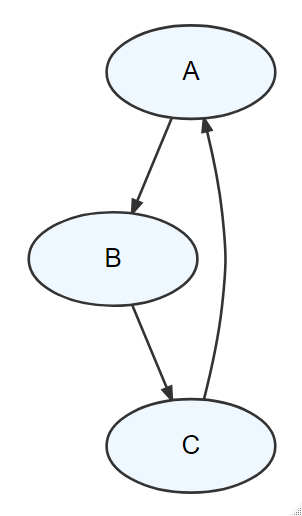 Figure 12.3: A graph that is NOT a DAG - it contains a cycle where you can return to any node by following the direction of the edges.
- All nodes represent random variables. They are drawn using ovals. By convention, a constant is also considered a random variable.
- All edges are pairs of random variables with a specified direction of ordering.\(^{**}\) By convention, the direction is from parent node to child node. ** While not always true, it is usually good to have edges reflecting a causal ordering. For example, it makes sense that an adventurous personality leads a person to prefer this new credit card. Rather than, the new credit card causing a person to become adventurous. Since we are using car model as a proxy for adventurous personality, it makes sense that car model is the parent node. Edges are drawn using arrows where the tail originates from the parent and the tip points to a child.
- Edges are uni-directional, they must only flow in one direction between any two nodes (i.e. directed).
- The graph is acyclic meaning there are no cycles. In other words, if you were to put your finger on any node and trace a path following the direction of the edges, you would not be able to return to the starting node. Figure 12.3 shows a cycle in a graph - it is NOT a DAG.
- Any child node’s probability distribution will be expressed as conditional solely on its parents’ values, i.e. \(P(child|parent(s))\); as we will see, this assumption is what enables more compact representations of joint distributions.
Figure 12.4: In this simple model, the probability distribution governing X will be a function of a specified value for Y.
*** The general rule for a probabilistic graphical model is that its joint distribution can be factored using the chain rule formula for DAGs where \(P(X_1, X_2, \ldots, X_n) = \prod_I P(X_i|Parents(X_i))\). Hence, to model any one random variable, we only have to model its relationship to its parents instead of modelling its relationship to all of the random variables included in the model.
Let’s use Figure 12.4 to review the probability distribution implications of an edge pointing into a node (requirement 5 from above). The one edge, \(Y \rightarrow X\), means that our uncertainty in \(X\) is measured using a probability function conditional on its parent - i.e. \(P(X|Y)\). Since there are no edges leading into \(Y\), it has no parents, its probability distribution is expressed \(P(Y)\). Now notice, with those two probabilities in place, we can recover the joint distribution, \(P(X,Y)\), based on the definition of conditional probability \(P(X,Y) = P(Y) \times P(X|Y)\). For reasons that will become more clear as we progress through this book, this is HUGE; edges and the absence of edges allow us to conveniently and compactly specify joint distributions.\(^{***}\)
*** See mathematicalmonk’s youtube video on how joint distributions are compactly represented using DAGs here: https://youtu.be/3XysEf3IQN4.
12.1.4 Aligning Graphical Models With Business Narratives
Edge presence and direction should reflect the narrative(s) your investigating. Figure 12.5 shows two alternate ways of structuring a graphical model with the same two nodes. If there are no edges between \(X\) and \(Y\), then the joint distribution is recovered via \(P(X,Y) = P(X) \times P(Y)\). In this case, the two random variables are independent and that is not a model structure consistent with the strategy we are exploring - we specifically hope that knowledge about car model impacts the probability someone wants the credit card. If the ordering of nodes for \(X\) and \(Y\) are reversed such that \(X\) is the parent of \(Y\), then the joint distribution would be recovered via \(P(X,Y) = P(X) \times P(Y|X)\). This math is suggestive of first determining whether someone gets the card and then, given that, determine the car model they drive. Since this does not reflect the narrative of our managerial story, this structure is deemed unsuitable. So in conclusion, the DAG structure of Figure 12.4 is the right one - not these alternatives; only Figure 12.4 reflects our narrative in how the random variables are related.
Figure 12.5: Two alternate graph structures: 1) X and Y are independent and 2) X is the parent of Y.
In subsequent chapters, we will combine our models with observed data to refine our probabilistic beliefs related to any DAG. As we observe some variables in the DAG, we refine our estimates in other variables. Joint distributions and their DAG representations are powerful - business narratives and data analysis gets linked.
12.2 Exercises
Graphical models are compact ways of recovering joint distributions. For example, take the following graph in Figure 12.6.
Figure 12.6: P(X,Y,Z) = P(Z) * P(Z|Y) * P(X)
To factor the joint distribution, \(P(X,Y,Z)\), one would write \(P(X,Y,Z) = P(X) * P(Y) * P(Y|Z)\).
Exercise 12.1 Write out the expression for the joint distribution implied by Figure 12.7
Figure 12.7: Write the factored expression P(X,Y,Z).
Exercise 12.2 Write out the expression for the joint distribution implied by Figure 12.8
Figure 12.8: Write the factored expression P(X,Y,Z).