Chapter 20 Decision Making
 Figure 20.1: The Ocean City boardwalk runs along this 2.5-mile long stretch of beach in Ocean City, MD.

Boardwalk Bathhouse’s business plan is to bring a private shower facility to the Ocean City, MD boardwalk. Currently, beachgoers visiting for the day have no way to wash off the saltwater and sand from a day at the beach. Nobody wants to get into their car or go out for dinner without a way of freshening up. We just need your help in deciding a location along the 2.5-mile long boardwalk (see Figure 20.1) to maximize our chances of success. Where should we put our bathhouse?
This is a typical decision under uncertainty and provides context for highlighting the BAW. When it comes to using the BAW for decision making, three key elements of the decision should be highlighted:
- An objective that we seek to improve. For example, “maximizing success” (we will learn to make this objective less ambiguous as we explore this decision further) and this provides the strategy component of the workflow.
- A decision or action which we want to make. This is the action that will be inspired by the BAW driven insight, such as “where to locate the business?”
- Uncertainty which makes decision making more difficult; and collecting data to reduce that uncertainty more valuable. For example, we have uncertainty as to “how many customers might visit any particular location?”
These three elements: objectives, decisions, and uncertainty are foundational elements of a field known as decision theory. Combining decision theory with other concepts from mathematics, computational statistics, and data visualization will allow us to be true gurus of business analytics; gurus who compel stategically-aligned actions that lead to better outcomes. This chapter will show you how.
20.1 Objectives
Of all the modelling assumptions we make traversing the business analytics bridge, the most important is that of choosing an objective. Effort spent refining a decision model is wasted when the objective is off course as comically depicted in Figure 20.2 (Ohmae 1989Ohmae, Kenichi. 1989. “Companyism and Do More Better.” Harvard Business Review 67 (1): 125–32.):
Figure 20.2: Quote by Kenichi Ohmae, Partner at McKinsey.

So, prior to embarking on any data-driven improvement effort, find or craft a strategy statement that serves as your navigational aid and documents your assumed objectives as an analyst (see Collis and Rukstad 2008Collis, David J, and Michael G Rukstad. 2008. “Can You Say What Your Strategy Is?” Harvard Business Review 86 (4). for details). Be vocal about this assumed strategy when talking with stakeholders; it will absolutely lead to informative and collaborative conversations. In addition, any unaddressed misalignment between you and your stakeholders may quickly lead to your dismissal from the meeting or the company. For example, a market-share-maximizing CEO might abhor your repeated focus on minimizing production costs when they feel maximizing customer acquisition or retention are much more important.
For Boardwalk Bathhouse, is maximizing weekly revenue or maximizing customer traffic the true goal of the business? Maybe maximizing profit is a better goal? Also, what about the probability of having a profit - maybe survival probability for this new business is also a key criteria? We will keep things simple and claim the business to be profit-maximizing. In more complex situations, we will often find a strong strategy statement provides time-saving clarity around which objectives or performance measures are important to look at.
20.2 Decisions
In your future, you will likely find yourself modelling decision policies that react to random inputs. We leave it up to the reader to explore how they might do this. In this book, we assume decision nodes have no random parent nodes and hence, decision nodes are completely deterministic and will take on only a single value. Figure 20.3 is a first pass at depicting the Boardwalk Bathhouse decision in a model. Decision nodes, shown as rectangles, are just like random variable nodes (ovals) with the exception that their value is controlled by an internal decision-maker. Hence, we get to choose the realization for a decision node and use that to feed information to the children nodes. In this case, we see how the location decision drives revenue, expenses, and subsequently, profit.
library(causact)
graph = dag_create() %>%
  dag_node("# of Hot Day Beachgoers") %>%
  dag_node(c("Rent by Location",
             "Beachgoer Location Probability"),
           obs = TRUE) %>%
  dag_node(c("Revenue","Expenses","Profit"),
           det = TRUE) %>%
  dag_node("Bathhouse Location",
           dec = TRUE) %>%
  dag_edge(from = c("# of Hot Day Beachgoers",
                    "Beachgoer Location Probability",
                    "Bathhouse Location"),
           to = "Revenue") %>%
  dag_edge(from = c("Bathhouse Location",
                    "Rent by Location"),
           to = "Expenses") %>%
  dag_edge(from = c("Revenue","Expenses"),
           to = "Profit")

graph %>% dag_render(shortLabel = TRUE,
                     wrapWidth = 15)
Figure 20.3: A draft generative model using a rectangle to indicate Boardwalk Bathhouse’s decision on where to locate.
The top-down narrative of Figure 20.3 is as follows. Boardwalk Beachhouse’s target customers are hot day beachgoers whose exposure to surf, salt, and sand will make them good candidates for wanting to get cleaned up. Since future weather and human behavior are unpredictable, the # of Hot Day Beachgoers is a random variable. These beachgoers spread-out across the 2.5 mile-long beach in a well-studied pattern represented as an observed data node named Beachgoer Location Probability. Using the # of Hot Day Beachgoers and Beachgoer Location Probability inputs, one can calculate Revenue as a function of these inputs and a given bathhouse location. Presumably, beachgoers closer to the Bathhouse Location will be more likely to contribute to revenue, but these details are currently omitted from the DAG. Similarly, Bathhouse Location also determines expenses, but further details are omitted from the DAG to keep things simpler.
In the above, code notice the expanded use of arguments in the
dag_node() function. Setting the
det,obs, or dec argument to
TRUE changes a node from being a standard random variable
to a deterministic, observed, or decision node, respectively.
Figure 20.3 reveals how we are mapping our location decision and other model inputs to the objectives we care about (revenue, expenses, and profit). Our strategy is similar to that of any other generative DAG in that we seek representative samples of unknown values; only this time, these representative samples are a function of our decision, e.g. Bathhouse Location. With representative samples in hand, we will pick the location that offers the best mix of objectives aligned with the firm’s strategy!
20.3 Uncertainty
Figure 20.4: Random variable node representing the number of hot-day beachgoers that can be expected in a year in Ocean City, MD.
The only uncertainty in Figure 20.3 is how many hot-day beachgoers will visit the beach during the year (shown in Figure 20.4). Although often possible and sometimes preferable, we will ignore exact mathematical specification of this uncertainty and simply look at uncertainty expressed as a representative sample, e.g. from a marginal, a joint distribution or some past data that we feel is representative of the future. For now, let’s pretend we are interpeting this as a representative sample from a posterior distribution. ** Crazy fact: Ocean city estimates its visitors using demoflush figures - a measurement of how many times Ocean City’s toilets were flushed. We can obtain a representative sample\(^{**}\) of # of hot-day beachgoers in a season from a vector built into the causact package named totalBeachgoersRepSample. A quick histogram of this representative sample is shown below:
library(tidyverse)
## ggplot needs tibble or dataframe input
beachgoerDF = tibble(
  totalBeachgoers = totalBeachgoersRepSample)
## above makes tibble from built-in
## totalBeachgoersRepSample vector
## plot results
beachgoerDF %>%
  ggplot() +
  geom_density(aes(x = totalBeachgoers),
               color = "navyblue", lwd = 2) +
  scale_x_continuous(labels = scales::comma_format())
Figure 20.5: Histogram generated from representative sample of the total number of hot-day beachgoers are expected on the beach in Ocean City, MD
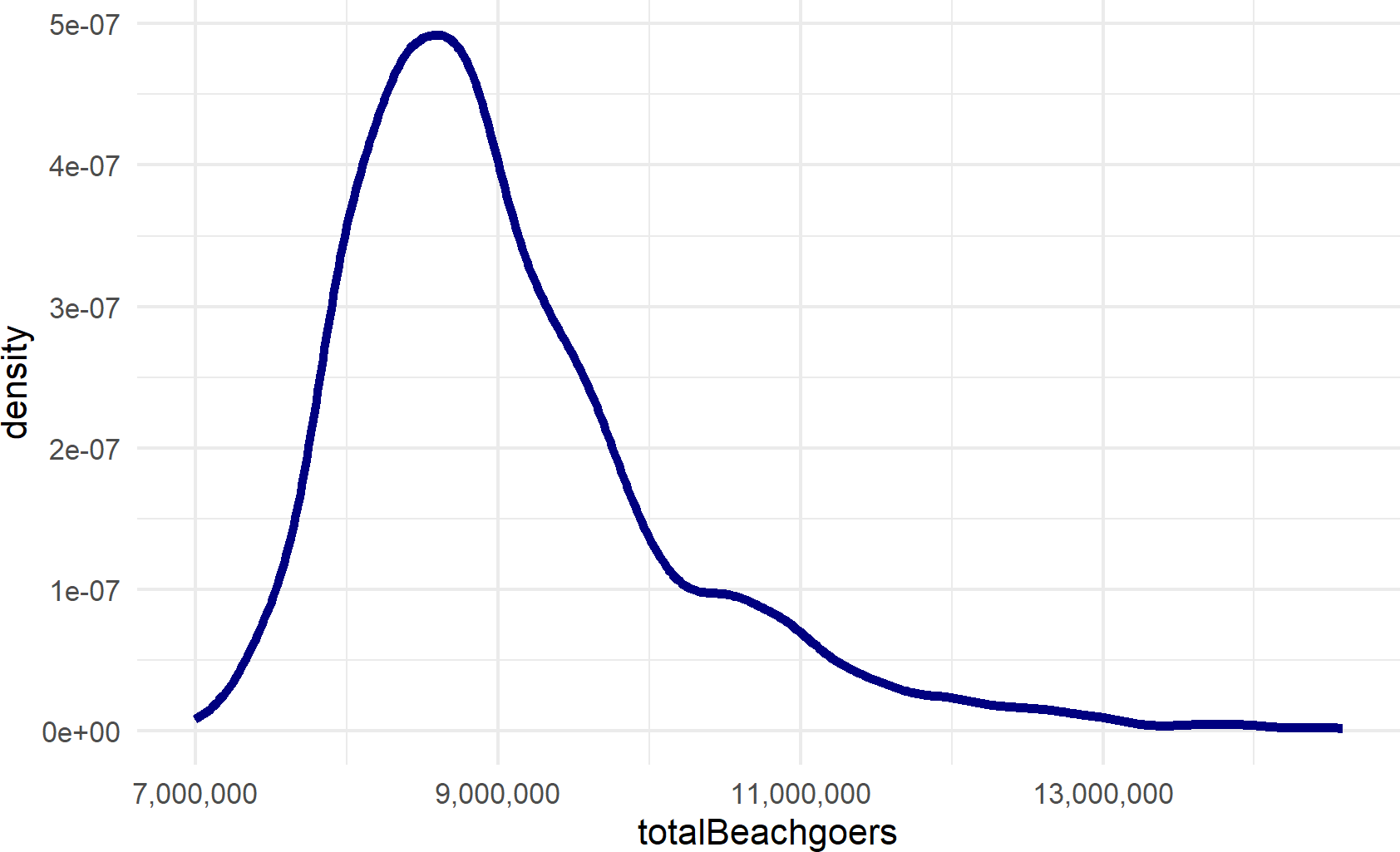
Figure 20.5 tells us to expect around 9,000,000 beach visitors (plus or minus a few million) every year to Ocean City. Boardwalk Bathhouse’s profitability will likely be very dependent on this uncertain number. That should not stop us from making a decision though, we boldy accept this uncertainty and use a generative recipe for analyzing our performance measures of interest.
20.4 Creating One Draw of a Generative Decision DAG
Figure 20.6: The generative DAG we are using to see how the bathhouse location decision impacts objectives like revenue, expenses, and profit.
The causact package is not developed enough to automate the simulation of generative models that include decisions. So, while we can use causact to go from prior to posterior and can use causact to create figures for communicating about models with decisions (as in Figure 20.6), we need to manually do the simulation from posterior to decision choice.
To aid our introduction, we make the following assumptions:\(^{**}\)
\(^{**}\) In a more accurate model, these assumptions would also be turned into distributions that reflect any uncertainty in those assumptions.
- 1% of beachgoers within 0.1 miles will become a customer of the bathhouse
- Each customer will pay $30.
Any changes to the above assumptions will alter our expectations and even alter the ideal action. While they should be explored in a real-world analysis, we will again ignore these additional details in favor of focusing on the translation from posterior uncertainty to decision making.
Following Figure 20.6 nodes from top to bottom, we will create a generative recipe for a joint realization (i.e. one draw of each node) of the generative DAG. Here’s how:
Generating a potential realization of revenue requires specification of the three parent nodes: 1) # of Hot Day Beachgoers, 2) Beachgoer Location Probability, and 3) Bathhouse Location. So, let’s create a recipe for calculating each of these parent nodes and then, subsequently calculating Revenue.
# of Hot Day Beachgoers is modelled using our representative sample (described above). To get a sample draw, we simply sample a single value from the representative sample as follows:
Beachgoer Location Probability is considered known and a table of location probability (beachgoerProb) by milemarker (mileMarker) is in the following built-in causact data frame:
## # A tibble: 26 × 2
##    mileMarker beachgoerProb
##         <dbl>         <dbl>
##  1        0           0.06
##  2        0.1         0.07
##  3        0.2         0.05
##  4        0.3         0.05
##  5        0.4         0.045
##  6        0.5         0.04
##  7        0.6         0.02
##  8        0.7         0.03
##  9        0.8         0.04
## 10        0.9         0.04
## # ℹ 16 more rows
Bathhouse Location is our decision, we get to choose this. Since the possible locations are already listed in beachLocProbDF, we will consider beachLocProbDF$mileMarker as our vector of possible locations choices. In decision theory, you would call the set of possible locations alternatives or actions. When reading more about decision theory, knowing these terms will be useful. Hence, we assume there are 26 possible alternatives, one location possibility every tenth of a mile.
Revenue is now a function of the three parents. Let’s make the function:
revenueFun = function(numBeachgoers,
                      locProbDF,
                      bathhouseLocation) {
  ## get number of potential customers exiting
  ## beach within 0.1 miles of bathhouse
  numPotentialCustomers = locProbDF %>%
    filter(abs(mileMarker - bathhouseLocation) <= 0.1) %>%
    mutate(custByMileMark = beachgoerProb * numBeachgoers) %>%
    summarize(potentialCustomers = sum(custByMileMark)) %>%
    pull(potentialCustomers)

  ## capturing 1% of potential customers on average
  ## means actual customers are a binomial rv
  ## hence, use the rbinom() function (see the
  ##representing uncertainty chapter for more info).
  numCust = rbinom(n = 1,
                   size = as.integer(numPotentialCustomers),
                   prob = 0.01)

  ## $30 per customer
  revenue = numCust * 30

  return(revenue)
}
Testing the revenue function above, we use numbers that let us easily verify the math. Assume there are 1,000,000 beachgoers, we know from beachLocDF that mile marker 0 will see around 13% of those beachgoers and 1% of those exiting beachgoers turn into customers (about 1,300 customers). At $30 per customer, revenue of around $39,000 is expected. Let’s see if the function works:
## [1] 39120Close enough for me. Yay!
Rent by Location is considered known and a table of rent expenses (beachgoerProb) by milemarker (mileMarker) is in the following built-in causact data frame:
## # A tibble: 26 × 2
##    mileMarker expenseEst
##         <dbl>      <dbl>
##  1        0       160000
##  2        0.1     160000
##  3        0.2     140000
##  4        0.3     140000
##  5        0.4     140000
##  6        0.5     140000
##  7        0.6     110000
##  8        0.7     110000
##  9        0.8     110000
## 10        0.9     110000
## # ℹ 16 more rows
Expenses is a function of its two parents. Let’s make the function:
expenseFun = function(locExpenseDF,bathhouseLocation) {
  ## get number of customers exiting at each mile marker
  ## by taking total # of beachgoers and using location
  ## probability to break the number down by mileMarker
  beachExpDF = locExpenseDF %>%
    filter(mileMarker == bathhouseLocation)

  return(beachExpDF$expenseEst)
}
Let’s make sure this function works. We know from beachLocDF that mile marker 0 will have expenses of $160,000. Testing this:
## [1] 160000And now this works too.
Last node to simulate in our top-down approach to computing a joint realization of the generative decision DAG is the profit node. We use a typical formula for profit:
\[ Profit = Revenue - Expenses \]
which we will model computationally in the next section where we simulate a draw from the generative decision DAG in Figure 20.6:
20.5 Simulating A Possible Outcome
With all the building blocks in place, we create a function that takes a potential decision and simulates one realization of revenue, expenses, and profit. It will return a single row as a data frame representing the draw.
generativeRecipe = function(bathhouseLocation) {
  numBeachgoers = getNumBeachgoers()
  locProbDF = beachLocDF %>%
    select(mileMarker,beachgoerProb)
  # bathhouseLocation is passed as input to function
  locExpenseDF = beachLocDF %>%
    select(mileMarker,expenseEst)
  rev = revenueFun(numBeachgoers,
                   locProbDF,
                   bathhouseLocation)
  exp = expenseFun(locExpenseDF,
                   bathhouseLocation)
  profit = rev - exp
  decDrawsDF = tibble(locDec = bathhouseLocation,
                      numBeachgoers = numBeachgoers,
                      rev = rev,
                      exp = exp,
                      profit = profit)
  return(decDrawsDF)
}
Let’s test it:
## # A tibble: 1 × 5
##   locDec numBeachgoers    rev    exp profit
##    <dbl>         <dbl>  <dbl>  <dbl>  <dbl>
## 1      1       8331000 171180 110000  61180
This also looks good. Yay again!!
20.6 Simulating a Range of Outcomes for All Possible Decisions
In this book, our representative samples often consist of 4,000
draws; this is the default value when running dag_numpyro()
which can be overridden using the num_samples argument (see
?causact::dag_numpyro). My rule of thumb for representative
samples is start with 4,000 draws and simulate results. If you repeat
this and the results change too much for your liking between repeated
simulations, then increase the number of draws. If the simulations are
taking too long, you can decrease the number of draws. Play with
repeated simulations of varying sizes until you are comfortable with
your own results. If you can’t get comfortable, then you will need to
find some mathematical or computational tricks to help.
Here we will use two for loops to get a representative sample of performance measures for each of the possible bathouse locations. The first loop, the outer loop, loops over possible decisions. The second loop, the inner loop, will then get 30 sample draws for a given decision. This code may take a minute or two; we have dramatically sacrificed computational speed in this chapter to keep the code intuitive (the end of this chapter offers guidance on making this simulation faster):
numSimsPerDec = 30 # number of sims per decision

## create empty dataframe to store results
decDrawsDF = tibble()

for (bathLoc in beachLocDF$mileMarker) {
  for (simNum in 1:numSimsPerDec) {
    drawDF = generativeRecipe(
      bathhouseLocation = bathLoc)
    decDrawsDF = bind_rows(decDrawsDF, drawDF)
  } # end inner loop
} # end outer loop
And then, we do a quick visual to inspect our decisions:
decDrawsDF %>%
  ggplot() +
  geom_point(aes(x=locDec,y=profit),
             size = 4,
             color = "navyblue",
             alpha = 0.5) +
  scale_y_continuous(labels = scales::dollar_format())
Figure 20.7: Representative samples of profit possibilities for all potential locations. Locating the bathhouse at mile marker 0.1 seems to be a clear winner - with smallest downside and largest upside potential.
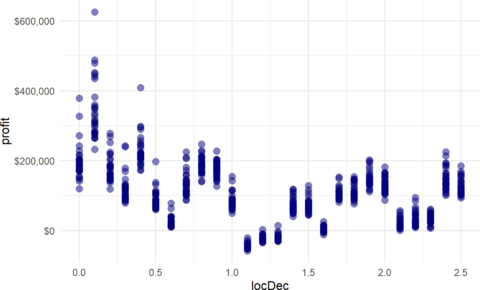
From visual inspection of Figure 20.7, there are certain locations that seem really good. However, be very skeptical of yourself - “can 30 points really capture a representative sample?” I would argue NO. We will see how to more quickly generate 1,000’s of samples in a subsequent section.
To demonstrate incorporating additional complexity into our simulation, let’s assume we only have $100,000 to invest, that disqualifies many of the locations. The change to incorporate this is common; manipulate the dataframe to eliminate the infeasible choices and then view the results (shown in Figure 20.8).
decDrawsDF %>%
  filter(exp < 100000) %>%
  ggplot() +
  geom_point(aes(x=locDec,y=profit),
             size = 4,
             color = "navyblue",
             alpha = 0.5) +
  scale_y_continuous(labels = scales::dollar_format())
Figure 20.8: Representative samples of profit possibilities for all potential locations that have expenses less than 100,000 dollars. Locating the bathhouse at mile marker 1.9 or 2.0 is now the best option.
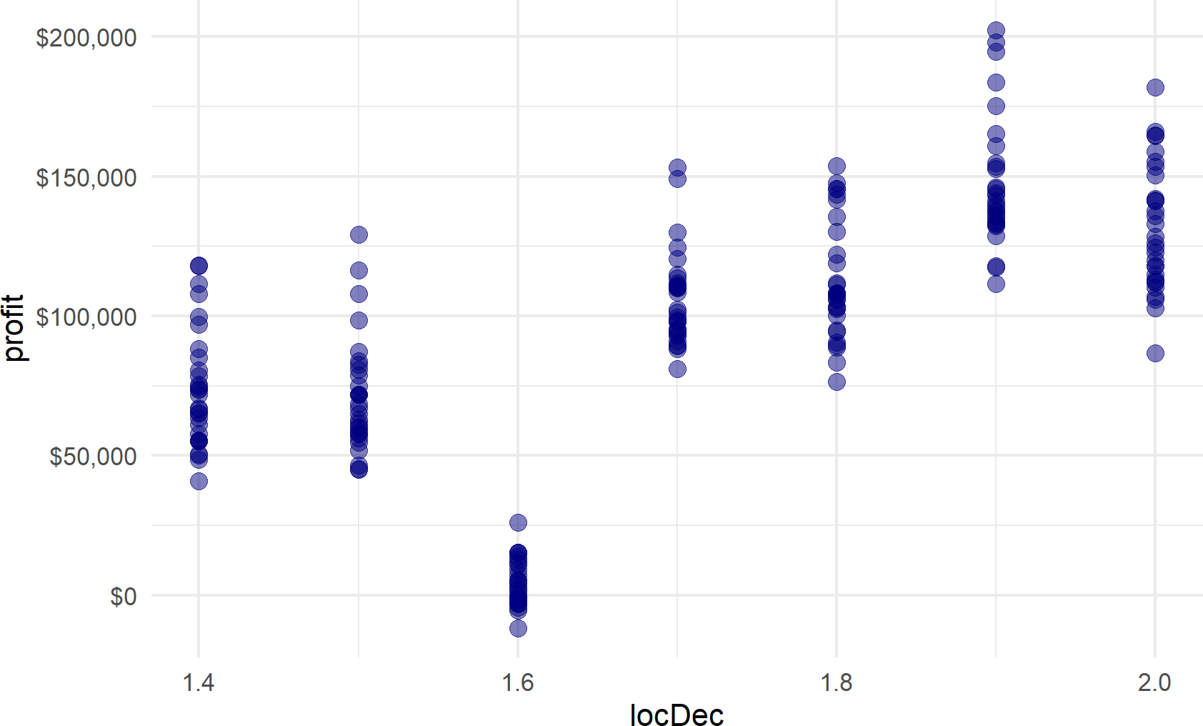
Under the budget constraint, locating at mile markers 1.9 (expenses of $96,000) or at mile marker 2.0 (expenses are $76,000) now provide the best outcomes.
20.7 Faster Code
In this section, we speed up the simulations above. Some guiding principles to make faster R code:
- Reduce the number of calculations: For us, this means we should not resimulate our one uncertainty node, # of Hot Day Beachgoers, for each decision. Since the random variable is independent of our decision, we can use the same representative sample for this value across all decisions.
- Avoid
forloops: In R,forloops are notoriously slow. However, new programmers find them more intuitive to use than other methods. For us, we useforloops without apology, but it is time to investigate other techniques when the loops seem to be slowing us down. Readers are encouraged to investigate thepurrrpackage for eliminatingforloops. See https://jennybc.github.io/purrr-tutorial/ for more on purrr. Additionally, and as is done below, often instead of dealing with one draw at a time, it becomes faster to work with a data frame of draws.dplyrverbs are speed-optimized, so performing functions on data frames is often faster than repeatedly calling one function to generate a draw of data and then combining all the rows. - Replace logical comaprisons with arithmetic when possible. Previously, we use
filter(abs(mileMarker - bathhouseLocation) <= 0.1)to determine if customers exiting a certain beach location were within range of the bathhouse. Below, this gets replaced with:
numPotentialCust = lag(numAtMileMarker, default = 0) +
  numAtMileMarker +
  lead(numAtMileMarker, default = 0))
where lead and lag get the potential customers from the 0.1 mile-higher mile marker and the 0.1 mile-lower mile marker and add them to the potential customers exiting the beach at the chosen bathhouse location.
We leave it to the reader to digest the below code one-line-at-a-time to see how the exact same results can be obtained with some small modifications to the preceding logic.
# take nSims as argument
fasterGenRecipe = function(nSims) {
  fastGenDF = tibble(
    simNum = 1:nSims,
    numBeachgoers =
      sample(totalBeachgoersRepSample,nSims)) %>%
    crossing(beachLocDF) %>%
    mutate(numAtMileMarker =
             numBeachgoers * beachgoerProb) %>%
    select(simNum,numAtMileMarker,
           mileMarker,expenseEst,numAtMileMarker) %>%
    group_by(simNum) %>% arrange(mileMarker) %>%
    mutate(numPotentialCust =
             lag(numAtMileMarker, default = 0) +
             numAtMileMarker +
             lead(numAtMileMarker, default = 0)) %>%
    ungroup() %>% arrange(simNum,mileMarker) %>%
    mutate(estRevenue =
             30 * numPotentialCust * 0.01) %>%
    mutate(profit = estRevenue - expenseEst) %>%
    select(simNum,mileMarker,profit,
           estRevenue,expenseEst)
  return(fastGenDF)
}
Figure 20.9 communicates potential profit ranges as blue bars and expenses as red text. This information captures the profit performance metric as well as conveying how much cash might be at risk if the business never got customers. New business owners may want to maximize profits under some budgetary prudence or constraints. This figure helps decision makers assess the trade-off. Interestingly, the most and least expensive locations are not necessarily the most and least profitable.
# separate out caption for readability of code
plotCaption =
  "Median Profit (dark point) and 90% Credible Interval"

fasterGenRecipe(4000) %>% group_by(mileMarker) %>%
        summarize(q05 = stats::quantile(profit,0.05),
                  q50 = stats::quantile(profit,0.50),
                  q95 = stats::quantile(profit,0.95),
                  expense = first(expenseEst)) %>%
        arrange(mileMarker) %>%
        ggplot(aes(y = mileMarker, yend = mileMarker)) +
        geom_linerange(aes(xmin = q05, xmax = q95),
                     size = 4, color = "#5f9ea0") +
        geom_point(aes(x = q50),
                   size = 4, color = "#11114e") +
        geom_text(aes(x = (expense - 120000),
                  label =
                    paste0("Annual Expense = ",
                           scales::dollar(expense))),
                  size = 3, color = "darkred") +
        labs(y = "Bathhouse Location Milemarker",
             x = "Annual Profit($)",
             caption = plotCaption) +
  scale_x_continuous(limits = c(-50000,450000),
                     labels = scales::dollar_format())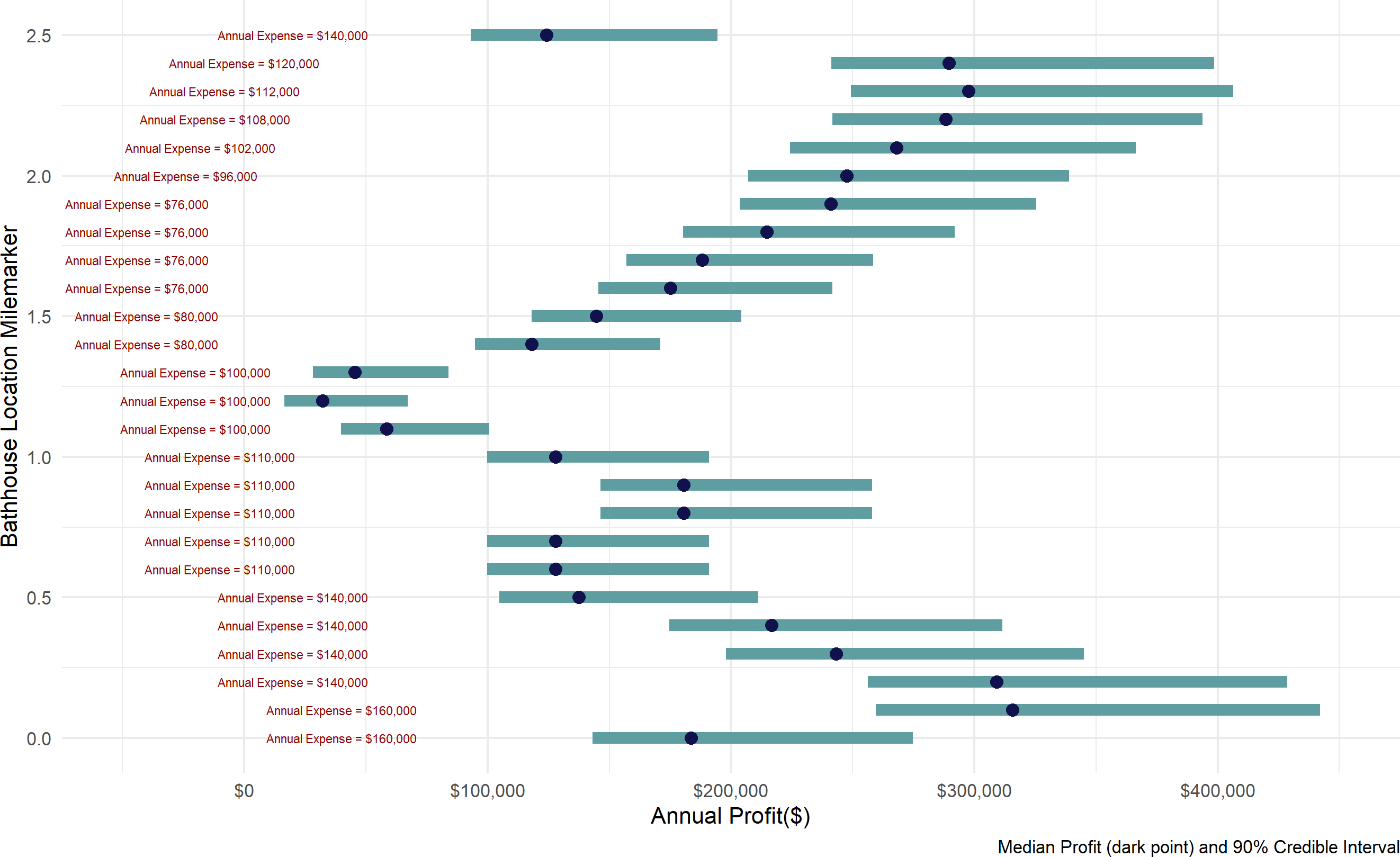
Figure 20.9: Summarizing a 4,000 draw representative sample to aid decision making. Mile markers 0.1, 0.2, 2.2, 2.3, and 2.4 are certainly worthy of consideration. And, if you want to minimize expenses, mile marker 1.9 provides great value in terms of return on investment.
In your own work, I encourage you to avoid presenting point estimates whenever possible. They are so incomplete in the information provided and will make your predictions look foolish as the most likely scenario is still rarely the scenario one sees play out in the business world. In Figure 20.9, declaring mile marker 1.5 to bring profit of $150,000 does not convey the real uncertainty where very different profit outcomes are possible - anywhere from $120,000 to over $200,000 are all very plausible outcomes.
20.8 Exercises
Exercise 20.1 In a famous model, known as the newsvendor model, a newsvendor must buy newspapers at the beginning of the day prior to knowing what demand for newspapers will be. Since demand is random, the newsvendor has to pick an order quantity which balances having too few newspapers (lost sales) and having too many newspapers (paid for newspapers that go unsold). Make the following assumptions about this model:
- OBJECTIVE: Choose a single order quantity \(q\) to maximize MEDIAN earnings over the 4,000 simulated draws of demand.
- Newsvendor buys newspapers for $1 and sells them for $2.
- Leftover newspapers at the end of the day are worthless.
- Newsvendor can only sell newspapers he has ordered, there is no midday resupply. Hence, if order quantity is \(q\), a representative sample of sales is given by
pmax(q,simDF$demand). - Assume a representative sample of future demand is given as
simDF$demandgenerated from the following code (details of the code are unimportant, we just need the output):
set.seed(123) # ensure we get same simulated future demand
num_samples = 4000
simDF = tibble(draw = 1:num_samples) %>%
  mutate(param1 = runif(num_samples,50,100),
         param2 = rgamma(num_samples,3,0.2),
         demand = as.integer(
           rnorm(num_samples,param1,param2))) %>%
select(demand)- The newspaper company only sells newspapers in multiples of 10. Thus, the newsvendor is considering ordering 50, 60 ,70 ,80, 90, or 100 newspapers each day.
Given the above, simulate expected MEDIAN profit for each order quantity. Which order quantity maximizes median profit and what is the median profit?
Exercise 20.2 Repeat the above exercise, except assume the newspaper company encourages larger orders of newspapers by buying back any unsold newspapers at the end of the day for $0.35. How many more newspapers does the newsvendor buy under this policy?