Chapter 23 Multi-Level Modelling

23.1 The Gym Data

Crossfit Gyms does not have alot of data, so let’s look at it a little bit.

## data from causact package that accompanies this book
library(causact)
library(tidyverse)
data("gymDF")  ## load into environment
gymDF  ## view the data

## # A tibble: 44 × 5
##    gymID timePeriod nTrialCustomers nSigned yogaStretch
##    <int>      <int>           <int>   <int>       <int>
##  1     1          1              32       7           0
##  2     2          1              56       4           0
##  3     3          1              42       1           0
##  4     4          1              58       9           0
##  5     5          1              84      44           0
##  6     1          2              38      14           0
##  7     2          2              68       7           0
##  8     3          2              42       3           0
##  9     4          2              64      13           0
## 10     5          2              72      33           0
## # ℹ 34 more rows

When thinking about visualizing this dataset, we need to understand that each row represents a particular gym (gymID) running one month of free trial classes. We use our dplyr trick of group_by and summarize

gymDF %>% group_by(gymID) %>%
  summarize(numberOfObservations = n())

## # A tibble: 12 × 2
##    gymID numberOfObservations
##    <int>                <int>
##  1     1                    5
##  2     2                    5
##  3     3                    5
##  4     4                    5
##  5     5                    5
##  6     6                    4
##  7     7                    4
##  8     8                    4
##  9     9                    3
## 10    10                    2
## 11    11                    1
## 12    12                    1

to discover that we have twelve unique gyms; the first 5 gyms give us five months of data each, while the next seven have less data (ranging from one to four free-trial months).

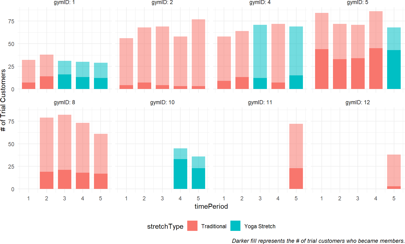
Since the small gymdDF data frame consists of only five variables, I am confident that I can map all five to aesthetics and show all the data using one plot command. After several iterations of plots (excluded here), here is one way to do that:

plotDF = gymDF %>%
  mutate(stretchType = 
           ifelse(yogaStretch == 1, 
                  "Yoga Stretch", 
                  "Traditional"))

ggplot(plotDF, 
       aes(x = timePeriod, #map time to x-axis
           y = nTrialCustomers, #map numTrials to y-axis
           fill = stretchType #map fill to stretch type
                  )) + 
  geom_col(width = 0.75, 
           alpha = 0.55) +  # use transparency
  geom_col(width = 0.75, 
           aes(y = nSigned)) + # different y-mapping
  facet_wrap(vars(gymID), labeller = label_both) + 
  theme_minimal(11) + 
  theme(plot.caption = 
          element_text(size = 9, face = "italic"),
        legend.position = "bottom") +
  ylab("# of Trial Customers") +
  labs(caption = 
         "Darker fill for # of sign-ups.")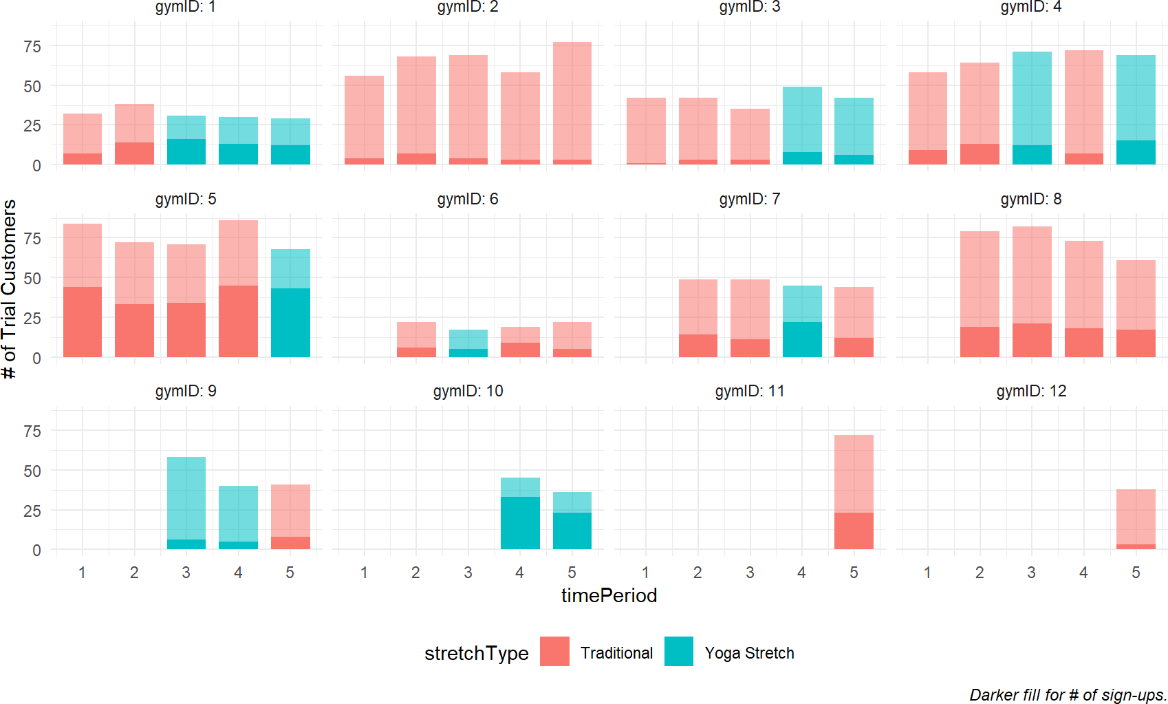

Figure 23.1: Plotting Cossfit Gyms success using trial memberships.

You can see from Figure 23.1 that the recruitment rate at each gym, represented by the proportion of dark fill to lighter fill, seems pretty consistent. However, there is apparent high variability across gyms. For example, gymID: 2 seems to be a consistently poor performer while gymID: 5 is somehow able to consistently make more conversions from free trials to paying memberships.

⊕Talking to the managers of these gyms to understand the differences in performance should be high on your to-do list, but for now (and because we do not have access to these managers), we will stick with the data that is available.

In terms of providing insight as to recruitment rates and the effect of extra yoga stretching (indicated by fill color), the visualization can only go so far. Yes, we can say gymID: 5 outperforms gymID: 2, but with only five months of data, how can we quantify our uncertainty about the differences? Additionally, yoga stretching seems to lead to better conversion rates, but how confident should we be given the seemingly small amounts of data?\(^{**}\) ⊕** Actually, the data size is not as small as you might think. While only 44 combinations of gym and time periods are observed, Crossfit Gyms has seen over 2,000 customers participate in a free trial.

23.2 Complete Pooling

⊕Complete pooling is a slight misnomer as we will have two distinct groups of observations. One group is with traditional stretching and the other yoga stretching.

The complete pooling model considers all observations to come from identical probability distributions; it does not differentiate based on gymID or timePeriod. Hence, all 44 observations behave as if they come from a single gym’s generative model. For this generative model, the unobserved parameter theta will be the only distinguishing feature. It takes one value for a traditional stretching class and another value for a yoga stretching class. ⊕The complete pooling model is shown for the contrast it provides in relation to other models you will see; it is an ill-advised model given that each gym clearly has a different baseline Signup Probability.

Under the complete pooling assumption, there is enough data that empirical estimates provide good probability estimates for the conversion rates by class type:

gymDF %>% group_by(yogaStretch) %>%
  summarize(nTrials = sum(nTrialCustomers),
            nSuccess = sum(nSigned)) %>%
  mutate(pctSuccess = nSuccess / nTrials)

## # A tibble: 2 × 4
##   yogaStretch nTrials nSuccess pctSuccess
##         <int>   <int>    <int>      <dbl>
## 1           0    1675      400      0.239
## 2           1     630      219      0.348

Here, we see that conversion rates seem to rise with the additional stretching from a base rate of 23.9% to 34.8%.

For illustration, Figure 23.2 shows the generative DAG for complete pooling. Despite not being a very good model for reasons we will see, it still provides a posterior with seemingly small uncertainty:

library(causact)
graph = dag_create() %>%
  dag_node("Number of Signups","k",
           rhs = binomial(nTrials,theta),
           data = gymDF$nSigned) %>%
  dag_node("Signup Probability","theta",
           child = "k",
           rhs = beta(2,2)) %>%
  dag_node("Number of Trials","nTrials",
           child = "k",
           data = gymDF$nTrialCustomers) %>%
  dag_plate("Yoga Stretch Flag","x",
           data = gymDF$yogaStretch,
           nodeLabels = "theta",
           addDataNode = TRUE) %>%
  dag_plate("Observation","i",
            nodeLabels = c("k","x","nTrials"))

graph %>% dag_render()

Notice that the graphical model has four random variables. Three of them are observed and enclosed in a plate labelled Observation i. This plate means that for each observation in our data (i.e. one of the 44 unique gym/time period rows in gymDF) , there are three observed random variables: 1) Number of signups (k), 2) Number of Trial Customers (nTrials), and 3) a flag indicating whether yoga stretch ws used or not (x). In contrast, the plate around Signup Probability, labelled Yoga Stretch Flag, indicates we have two random variables for Signup Probability: 1) a Signup Probability for traditional Stretching (i.e. probability when x=0) and 2) a Signup Probability for yoga Stretching (i.e. probability when x=1). In other words, all gyms have the same two success probabilities associated with them; we call this complete pooling of the gyms as according to the model, each gym is identical. We know this is a ridiculous assumption from visualizing the data in Figure 23.1, but we use this to illustrate that there are very meaningful assumptions tied to each graphical model we make. ⊕Note that we do not specify distributions for the number of trials or the yoga stretch indicator. We assume these are always given, and hence are not interested in measuring our uncertainty in these variables. If we did want to predict values for these - for example, how many customers will sign up for a free trial? - then, we would model them statistically.

Computationally, we go through the standard process to get our posterior:

drawsDF = graph %>% dag_numpyro()

And then, we look to Figure 23.3 to analyze our posterior draws. Estimated signup probability for yoga stretching (about 35%) seems to range higher than without yoga (less than 25%).

drawsDF %>% dagp_plot() 

Figure 23.3: Posterior uncertainty in two success probability parameters. theta0 for no yoga and theta1 for with yoga.

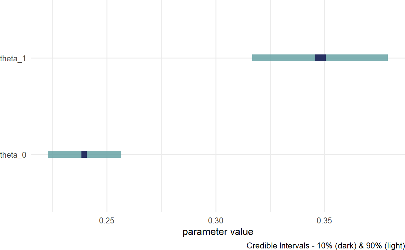
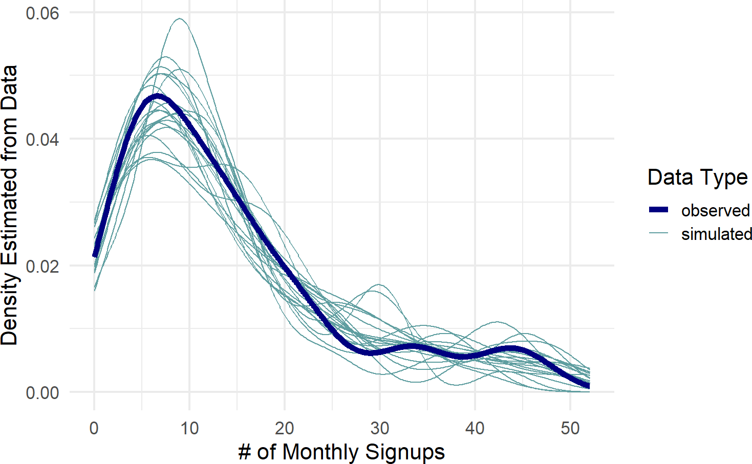
Perhaps, the fact that these probability estimates align with the emprical estimates (above) should seem comforting, but there is something sinister lurking in our model choice. Recall that our visual sensibilities applied to Figure 23.1 have already noticed differences among the gyms. So, it should be expected that we are not accurately modeling the data generation process when ignoring these differences. By performing a posterior predictive check, ⊕The posterior predictive check uses similar code as seen in the posterior predictive check chapter. Yes, it is a little tedious, but we are at the limits of what has been developed for this type of computing. we see how looking at this overly simple complete pooling model fails to capture some of the patterns observed in the actual data.

## get DF of observed data and remove target measure
simDF = gymDF %>% select(-nSigned)

## get 20 random draws of posterior
paramsDF = drawsDF %>%
  slice_sample(n=20) %>%
  mutate(sampDrawID = row_number()) ## add id to track

## get all combinations of observed explanatory
## variables and the parameter draws
simDF = simDF %>%
  crossing(paramsDF)
## 44 observations * 20 sample draws = 880 rows

## if no yoga, then theta_0.  If yoga, then theta_1
simPredDF = simDF %>%
  mutate(signupProb = 
           ifelse(yogaStretch == 0, 
                  theta_0, theta_1)) %>%
  mutate(nSigned = rbinom(n = n(),
                          size = nTrialCustomers,
                          prob = signupProb))  

obsDF = tibble(obs = gymDF$nSigned)

colors = c("simulated" = "cadetblue", 
           "observed" = "navyblue")

## make plot
ggplot(simPredDF) +
  stat_density(aes(x=nSigned, 
                   group = sampDrawID,
                   color = "simulated"),
               geom = "line",  
               position = "identity") +  
  stat_density(data = obsDF, aes(x=obs, 
                                 color = "observed"),
               geom = "line",  
               position = "identity",
               lwd = 2) +
  scale_color_manual(values = colors) +
  labs(x = "# of Monthly Signups",
       y = "Density Estimated from Data",
       color = "Data Type")

Figure 23.4: Posterior predictive check to see if model is capable of capturing the variability inherent in the observed data.

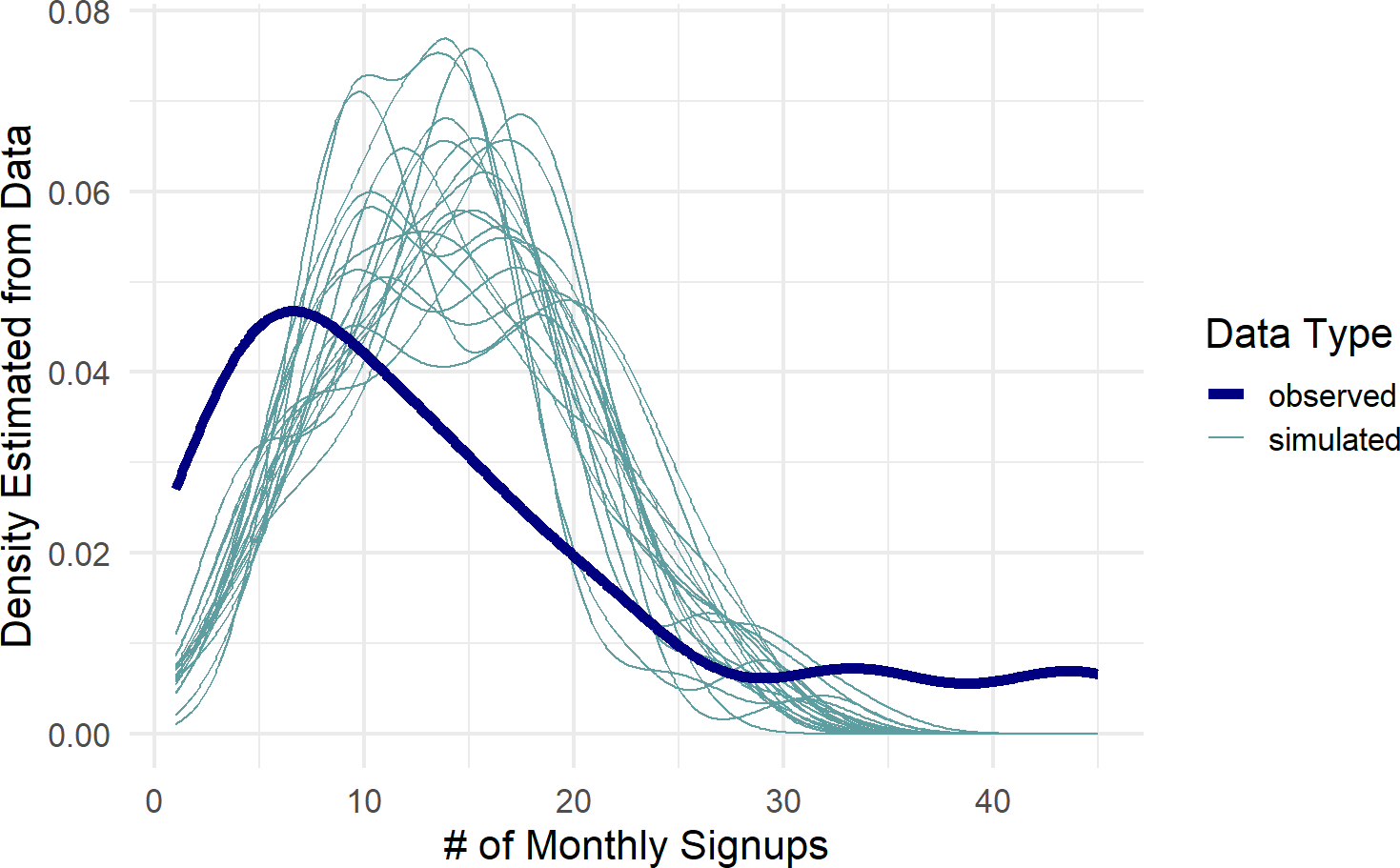
Figure 23.4 shows the observed data density plot across gyms as represented by the dark blue line. This observed distribution is not captured by the spaghetti lines, i.e. predicted distributions from the posterior, none of the 20 sample predicted distributions come close to mimicking the behavior seen in the actual data. This is a clear signal we are not modelling something right; namely each gym will have some differences in recruiting probabilities, and hence, produce more varied amounts of success than suggested by the complete pooling model.

23.3 No Pooling

The no pooling model treats each gym as distinct completely independent entities, i.e. the Crossfit Gym franchise has no overarching effect on success probabilities. ⊕The no pooling model is shown for the contrast it provides in relation to other models we will look at; it is an ill-advised model when you have small data and transferable learning. We will assume learning about one gym’s success rate should impact our opinion about another gym’s success rate - we do not want each gym to be distinct. Thus, learning about one gym’s success in recruiting tells us nothing about the population of gyms or any other specific gym.

On our path to modelling the effects of yoga, we are going to refine our previous generative DAG to get closer to the business narrative. Specifically, we want to ensure a direct modelling of the effect of yoga stretching.

We are going to assume there is a base-level of recruitment at each gym and that yoga stretching provides some deviation from the base. If we were to model the deviation as a probability deviation, say yoga increases recruitment probability 20%, than its possible that forecasting the effect of yoga at a gym with a base recruitment rate of 85% leads to 105% sign-up probability - this is a problem as probability of signup cannot be over 100%.

To remedy this, we use a linear predictor as input into an inverse logit link function; it ensures signup probability draws are actually probability values between 0 and 1. This new generative story with base recuitment probability and deviation for yoga is reflected in the DAG of Figure 23.5.

Figure 23.5 has slope and intercept terms that are not directly understandable - they go through an inverse logit function before we see their impact on a node that we can understand. To understand the prior on these terms (or any prior), we simulate how its values are transferred to a parameter of interest, in this case that parameter is signup probability.

23.3.1 Using Simulation To Help Choose Priors

Unfortunately, I am always writing custom code to explore the effect of priors on the children of transformed linear predictors. This part of the BAW process will be accelerated in future versions of causact. Until then, here is some code to help find a good alpha:

library(tidyverse)
numSims = 10000

## guess at distribution and params for alpha
## let's say alpha ~ normal(0,10) was my first guess
## then simulate effects on theta.  Do they mimic
## your uncertainty in theat without data?  If no,
## iterate with a different guess. After 
## many iterations I settled on normal(-1,1.5)
## below code gets repsample of theta for this prior
simDF = tibble(alpha = rnorm(n = numSims, 
                             mean = -1., 
                             sd = 1.5))

simDF = simDF %>%
  mutate(y = alpha) %>% ##follows DAG
  mutate(theta = 1 / (1 + exp(-y)))  ## inv logit

## plot implied theta distribution
ggplot(simDF) +
  geom_density(aes(x=theta),fill = "cadetblue") 

Figure 23.6: The final choice of prior, alpha ~ N(-1,1.5), it is mildly informative, but open to all sorts of theta possibilities.

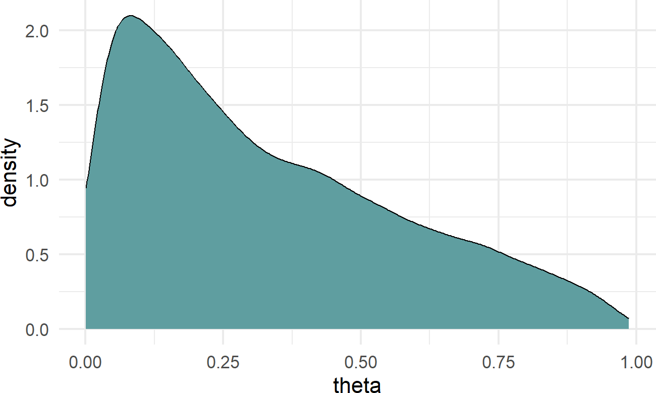
⊕Don’t obsess over getting priors just perfect. By having them close enough to your beliefs and open to things against your initial beliefs, you will find the data plus prior to get you insights where they exist and avoid false insights where they don’t.

Figure 23.6 is the result of many iterations of looking at the effect of changes in alpha’s prior on success probability theta. I stopped at \(N(-1,1.5)\) because it reflected my mild belief that sign-up probability will be smaller than 50%, but should also remain open to any possible value. I am also comfortable with the hump of probability around 10%, that sounds like a good mode for recruiting.

Your prior should be open to changing its mind, but it should also reflect assumptions you are willing to make. Don’t be afraid to have mildly informative priors, they do not all need to be uniform. This will protect you from bad decisions when there is not alot of data to inform the posterior.

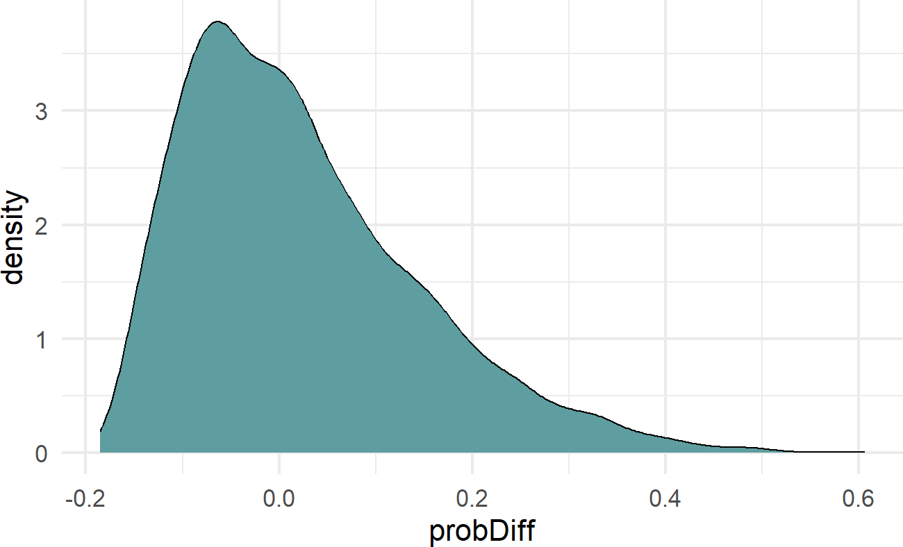
A similar exercise is done for the prior on \(\beta\). Recognizing that stretching is most likely going to have a small effect. I run the following code to find my prior:

library(tidyverse)
numSims = 10000

## guess at distribution and params for beta
## since beta is deviation from base rate alpha
## assume a base rate and then, see effects
## mean should absolutely be zero to indicate no prior
## preference for whether yoga is helpful
## let the data tip the scales
## sd should be smaller than that used for alpha
baseRate = 0.20  ## assumed for now

## logit function 
## input: probability, 
## output: linear Predictor
## inverse of the inverse logit function
## linearPredictor = log(probability / (1-probability))
alpha = log(baseRate / (1 - baseRate))

simDF = tibble(alpha = alpha,
               beta = rnorm(n = numSims,
                            mean = 0,  
                            sd = 0.75))

simDF = simDF %>%
  mutate(yNoYoga = alpha) %>%
  mutate(yWithYoga = alpha + beta) %>%
  mutate(thetaNoYoga = 1 / (1 + exp(-yNoYoga))) %>%
  mutate(thetaWithYoga = 1 / (1 + exp(-yWithYoga))) %>%
  mutate(probDiff = thetaWithYoga - thetaNoYoga)

## plot implied theta distribution
ggplot(simDF) +
  geom_density(aes(x=probDiff),fill = "cadetblue") 

Figure 23.7: The final choice of prior, beta ~ N(0,0.75), it is mildly informative in that small probability differences due to yoga are more likely than large deviations.

23.3.2 The Posterior Distribution

After tuning the statistical model part of our generative DAG (Figure 23.5), we create the posterior seen in Figure 23.8.

graph = dag_create() %>%
  dag_node("Number of Signups","k",
           rhs = binomial(nTrials,theta),
           data = gymDF$nSigned) %>%
  dag_node("Signup Probability","theta",
           child = "k",
           rhs = 1 / (1+exp(-y))) %>%
  dag_node("Number of Trials","nTrials",
           child = "k",
           data = gymDF$nTrialCustomers) %>%
  dag_node("Linear Predictor","y",
           rhs = alpha + beta * x,
           child = "theta") %>%
  dag_node("Yoga Stretch Flag","x",
           data = gymDF$yogaStretch,
           child = "y") %>%
  dag_node("Intercept","alpha",
           rhs = normal(-1,1.5),
           child = "y") %>%
  dag_node("Yoga Slope Coeff","beta",
           rhs = normal(0,0.75),
           child = "y") %>%
  dag_plate("Gym","j",
            nodeLabels = c("alpha","beta"),
            data = gymDF$gymID,
            addDataNode = TRUE) %>%
  dag_plate("Observation","i",
            nodeLabels = c("k","x","j",
                           "nTrials","theta","y"))

drawsDF = graph %>% dag_numpyro()

drawsDF %>% dagp_plot()

Figure 23.8: Posterior distribution for alpha and beta.

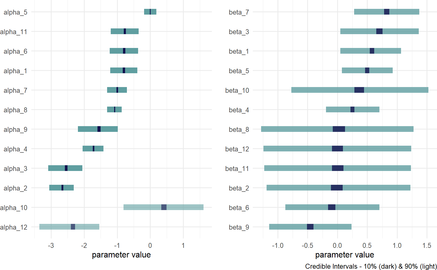
Visually inspect the posterior estimates of Figure 23.8. Recall that these are components of a linear predictor (i.e. \(\alpha + \beta x\)). If the linear predictor is zero, that corresponds to a probability of 50% (see Figure 23.9). Hence, values for \(\alpha < 0\) would imply base conversion rates less than 50%. Values for \(\beta\) indicate whether that base probability should be adjusted up or down; \(\beta < 0\) implies a negative effect for the yoga stretching routine and \(\beta > 0\) indicates that the effect is positive.

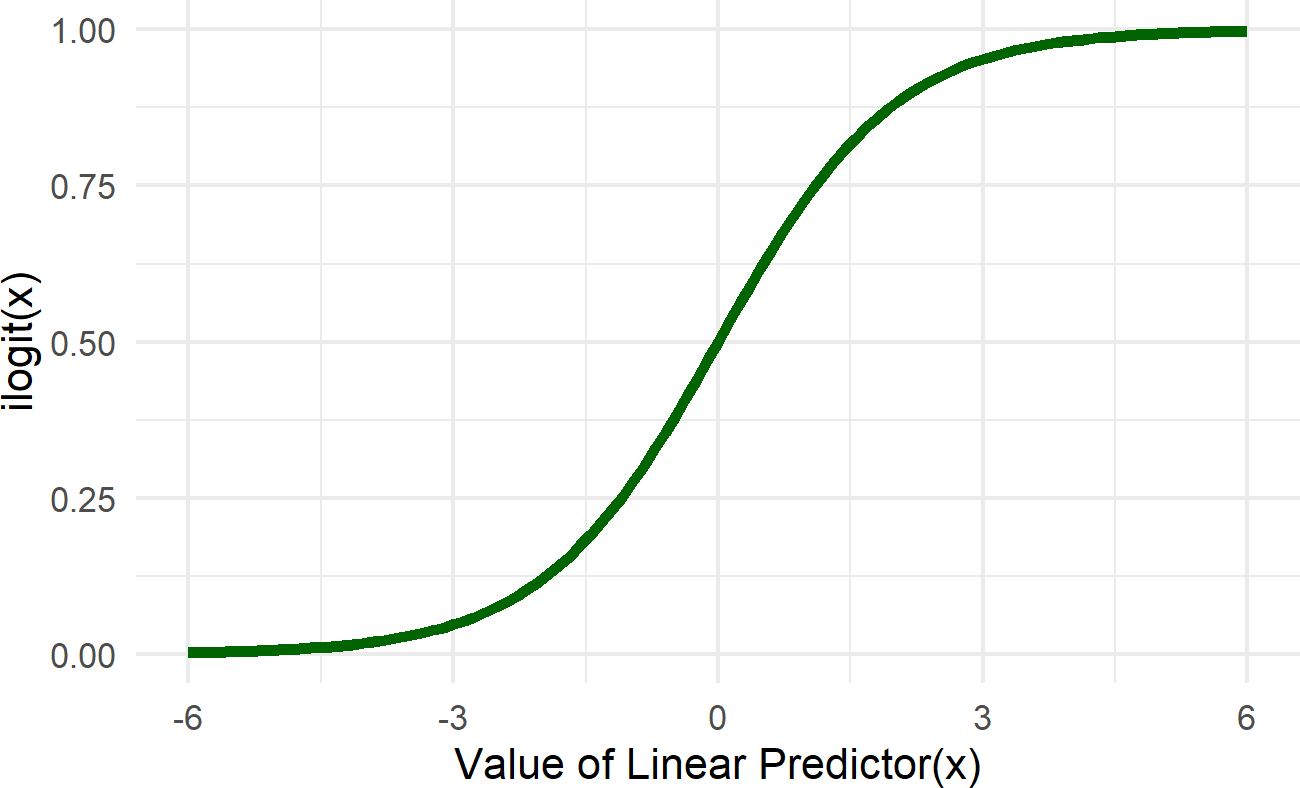Figure 23.9: Graph of the logistic function (aka the inverse logit function). The linear predictor in our case is alpha + beta * x. The role of the ilogit function is to map this linear predictor to a scale bounded by zero and one. This essentailly takes any number from -infinity to infinty and provides a probability value as an output.

Comparing Figure 23.8 with plots of the gym data in Figure 23.10, notice how the posterior estimates correspond with your expectations. The \(\alpha\) values with the smallest credible intervals are for gyms that have the largest number of trial customers participating in trials with traditional stretching (i.e. gyms 2, 5, and 8). Similarly, the \(\beta\) values with the smallest credible intervals are for gyms that have the largest number of trial customers participating in Yoga stretching classes (i.e. gyms 1 and 4). The opposite is also observable. Gyms lacking data for traditional stretching have wide credible intervals for \(\alpha\) (e.g. gym 10) and gyms lacking data for yoga stretching do not improve on the prior uncertainty in \(\beta\) (e.g. gyms 11 and 12).

Figure 23.10: Illustration of 8 out of the 12 gyms data.

This no pooling model is not terrible in the sense that each gym gets statistically modelled. Let’s do some challenging data manipulation (go through it slowly) and do a posterior predictive check:

## get DF of observed data and remove target measure
simDF = gymDF %>% select(-nSigned)

## get 20 random draws of posterior
paramsDF = drawsDF %>%
  slice_sample(n=20) %>%
  mutate(sampDrawID = row_number()) 

## when data like gym_id is in the name of column 
## headings, e.g. alpha_4,
## we use the tidyr package pivot_longer function 
## to turn headings into data
## and extract the gymID information from the heading
tidyParamDF = paramsDF %>% 
    pivot_longer(cols = -sampDrawID) %>%
    mutate(gymID = str_extract(name, '[0-9]+')) %>%
    mutate(gymID = as.integer(gymID)) %>%
    mutate(paramName = str_extract(name, '[:alpha:]+'))

## now we get explanatory variable info 
## combined with relevant params
simDF = simDF %>% left_join(tidyParamDF, by = "gymID") 
## 44 observations * 2 params per row * 20 sims 
## = 1,760 rows

## get relevant alpha and beta on same row
simPredDF = simDF %>%
  pivot_wider(id_cols = gymID:sampDrawID,
              names_from = paramName,
              values_from = value)

## if no yoga, then y=alpha.  If yoga, then y=alpha+beta
simPredDF = simPredDF %>%
  mutate(y = ifelse(yogaStretch == 0, 
                    alpha, alpha+beta)) %>%
  mutate(theta = 1 / (1 + exp(-y))) %>%
  mutate(nSigned = rbinom(n = n(),
                          size = nTrialCustomers,
                          prob = theta))

obsDF = tibble(obs = gymDF$nSigned)

colors = c("simulated" = "cadetblue", 
           "observed" = "navyblue")

## make plot
ggplot(simPredDF) +
  stat_density(aes(x=nSigned, 
                   group = sampDrawID,
                   color = "simulated"),
               geom = "line",
               position = "identity") +
  stat_density(data = obsDF, aes(x=obs, 
                                 color = "observed"),
               geom = "line",  
               position = "identity",
               lwd = 2) +
  scale_color_manual(values = colors) +
  labs(x = "# of Monthly Signups",
       y = "Density Estimated from Data",
       color = "Data Type")

Figure 23.11: Posterior predictive check for the no-pooling model comparing the observed data to data generated using 20 different draws from the posterior distribution.

⊕Splitting strings or text like we do to extract the gymID from the coefficient names like alpha_10 involves the use of regular expressions. I have no memory for this information and need to google it everytime. Here is a helpful link for more info: https://stringr.tidyverse.org/articles/regular-expressions.html.

This posterior predictive check looks really good. Yet, Figure 23.8 revealed there are credible intervals which can be made smaller; uncertainty bands can be narrowed for gym’s missing one type of class. We know, from previous observation at all the gyms, that yoga’s effect seems small. Hence, the wide \(\beta\) uncertainty bands are not warranted. Going the other way, we should have more confidence in gym 10’s recruitment rate (\(\alpha_{10}\)). Gym 10 is a star performer and I do not think dropping the yoga-stretch will lead to enormous drops in rate. Overall, I think we should agree that learning about one gym might tell us something about another gym. In fact, I would argue that learning about 12 gym’s should tell us what we might expect when the next 100 gyms are opened. The next model explores this and shows us we can do better.

23.4 Partial Pooling

The partial pooling model imagines that the Crossfit Gyms business model produces gyms with similar characteristics. Some gyms will do better than average and some gyms will do worse, but there is some relationship between each gym’s performance. In this case, learning about one gym’s success in recruiting provides information about that gym as well as the entire population of Crossfit gyms.

To accomodate this structure (i.e. known as hierarchical or multi-level structure), we add parent nodes to the gym-level coefficients in the previous generative DAG (stored in graph) and change the statistical model for those gym-level coefficients as well. The partial pooling model generative DAG (graph2) can be specified as:

library(causact)

graph2 = dag_create() %>%
  dag_node("Number of Signups","k",
           rhs = binomial(nTrials,theta),
           data = gymDF$nSigned) %>%
  dag_node("Signup Probability","theta",
           child = "k",
           rhs = 1 / (1+exp(-y))) %>%
  dag_node("Number of Trials","nTrials",
           child = "k",
           data = gymDF$nTrialCustomers) %>%
  dag_node("Linear Predictor","y",
           rhs = alpha + beta * x,
           child = "theta") %>%
  dag_node("Yoga Stretch Flag","x",
           data = gymDF$yogaStretch,
           child = "y") %>%
  dag_node("Gym Intercept","alpha",
           rhs = normal(mu_alpha,sd_alpha),
           child = "y") %>%
  dag_node("Gym Yoga Slope Coeff","beta",
           rhs = normal(mu_beta,sd_beta),
           child = "y") %>%
  dag_node("Avg Crossfit Intercept","mu_alpha",
           rhs = normal(-1,1.5),
           child = "alpha") %>%
  dag_node("Avg Crossfit Yoga Slope","mu_beta",
           rhs = normal(0,0.75),
           child = "beta") %>%
  dag_node("SD Crossfit Intercept","sd_alpha",
           rhs = uniform(0,3),
           child = "alpha") %>%
  dag_node("SD Crossfit Yoga Slope","sd_beta",
           rhs = uniform(0,1.5),
           child = "beta") %>%
  dag_plate("Gym","j",
            nodeLabels = c("alpha","beta"),
            data = gymDF$gymID,
            addDataNode = TRUE) %>%
  dag_plate("Observation","i",
            nodeLabels = c("k","x","j",
                           "nTrials","theta","y"))

graph2 %>% dag_render()

Take note of Figure 23.12’s top row of random variables characterizing the population of gyms. Think of the first two nodes as characterizing the base conversion rate for the population of crossfit gyms - one represents an expectation of any single gym’s intercept and the other represents how much deviation should be expected between the intercept’s of all the gyms. For example, a high mu_alpha and a small sd_alpha would suggest any randomly chosen Crossfit gym will have a high base-level probability for membership sign-ups and additionally, no matter which gym is chosen, its likely to have a similarly high base-level probability.

For priors, we used our previous prior for gym-level intercept to now be the prior for its parent, mu_alpha which is the expected base intercept for any Crossfit gym. The standard deviation component, sd_alpha, uses a uniform distribution that is twice the standard deviation prior for mu_alpha; chosen so the variation in base conversion rates will be on a similar scale to our own uncertainty in the corresponding mean, i.e. mu_alpha.

The next two nodes atop Figure 23.12 suggest that every gym’s slope coefficient for yoga is drawn from a distribution characterized by an average effect of yoga stretching for any Crossfit gym, mu_beta, and a standard deviation, sd_beta measuring how likely any individual gym’s effect might deviate from the average. Priors are chosen as was done for the first two nodes. ⊕Note that standard deviations of the Crossfit population parameters control how much pooling of information takes place. Larger standard deviations indicate a process where the population seems to have little impact on each individual gym. Whereas smaller standard deviations suggest that each gym has very similar characteristics.

Through these population parameters, each gym’s \(\alpha_j\) and \(\beta_j\) are related; in cases of minimal gym data, the population parameters will be very important in estimating gym performance, conversely, in cases a gym shows strong deviation from the population parameters over a lot of trial customers, then these population parameters will get ignored.

⊕Prior distribtuions placed on parameters are often called hyperparameters. Feel free to just call them priors on priors if you like that better.

With generative DAG in place, we can compute and visualize the posterior in the standard way.

drawsDF = graph2 %>% dag_numpyro()
drawsDF %>% dagp_plot()

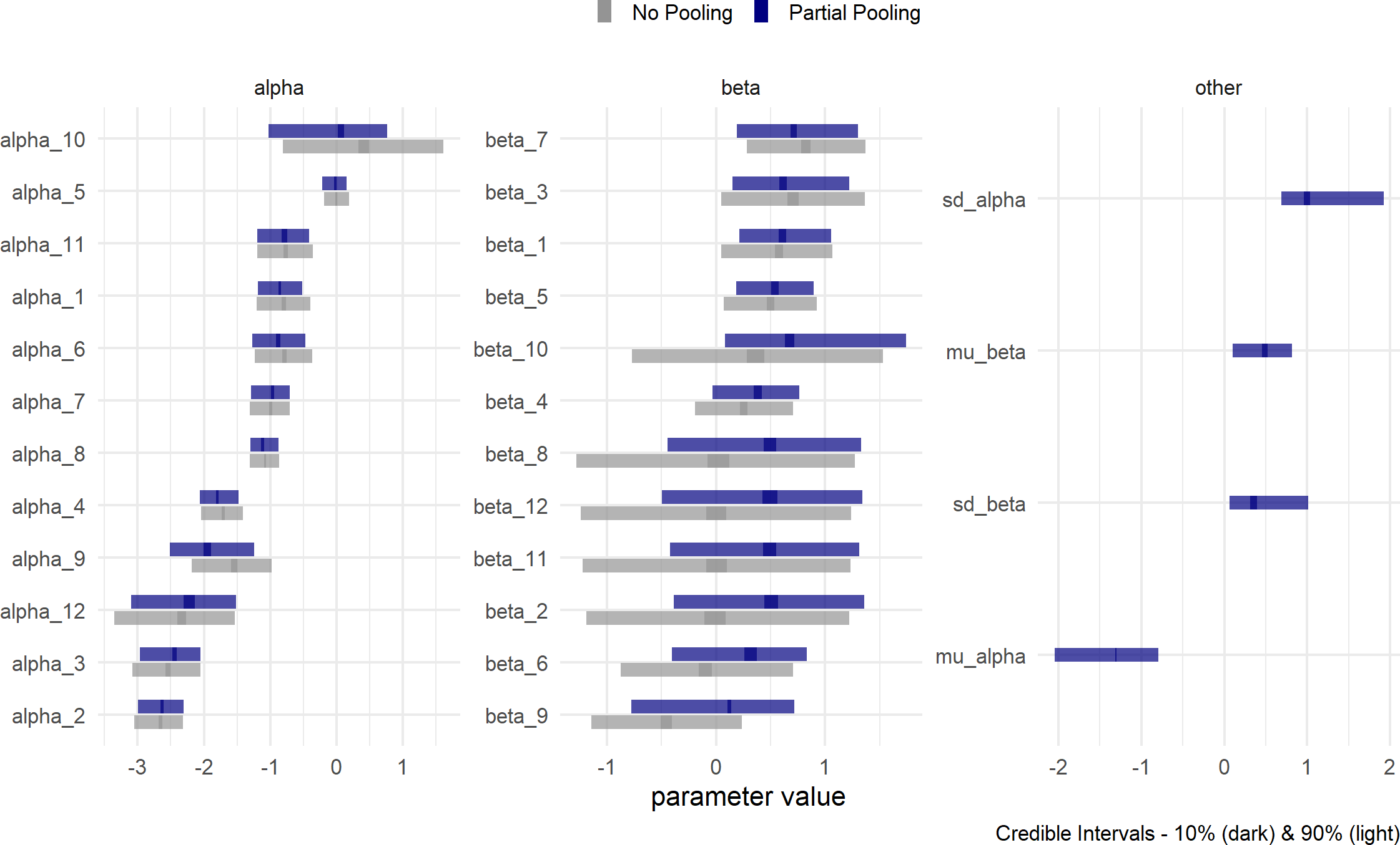
Figure 23.13: Partial Pooling - Estimates for the parameters of the generative model where each gym’s parameters are related. I like to think of the relation being due to the Crossfit hyperparameters (i.e. priors on parameters) giving birth to the gym-level parameters.

Figure 23.13 shows a slightly different snapshot of the posterior distribution. In addition to the partial pooling posterior, the previous no-pooling posterior is also put on the graph for comparison. This will help us see what gains are made (or not) by adding the four hyperparameters (i.e. mu_alpha,mu_beta,sd_alpha,sd_beta)

Visually comparing the estimates of the two models shown in Figure 23.13 helps us learn how to think about the multi-level model’s (i.e. partial pooling) interpretation:

• Uncertainty interval widths have shrunk; especially for gym/stretching combinations that have yet to be seen. For example, gym10 has only two observations, both yoga, no traditional stretching observations. Now look at the change in \(\alpha_{10}\), the base conversion rate parameter without yoga. Its a narrower interval than with no pooling. The narrowness is because we have learned about the effects of yoga from the other gyms and hence, can reason better about this unobserved base rate. This base rate remains high because we have also learned that differences due to yoga are never that dramatic.
• There is increased confidence that yoga stretching would be effective at each gym. Look at the rightward shift of most of the partial pooling beta estimates. Also, mu_beta, the average effect of yoga is clearly greater than zero; hence, it seems like a good idea for Crossfit to promote yoga.
• Not all gym’s are equal. Looking at gym 9 where there are 3 time periods of observations - one with traditional stretching that seemed better than the others. From the partial-pooling posterior, you see a rightward shift of beta_9 as compared to the no-pooling model because we’ve learned that yoga works at other gyms. The uncertainty interval is clearly both positive and negative indicating we need more data to confidently dismiss or accept the idea of yoga.
• Both alpha and beta intervals in the partial pooling model often (but not always) get pulled towards their means, mu_alpha and mu_beta respectively. Because we are sharing information through these parents, their impact gets felt at the gym level - especially in cases of gym’s without much data. For example, gym 12 only has one time period of observation, so both alpha_12 and beta_12 intervals are pushed towards the expected values of their parent nodes. Gym 5 has alot of data and as a result does not respond to these parental node influences.
• The interval for sd_alpha being away from zero suggests that there is alot of deviation between gyms in terms of average expected base conversion rate. Recruitment rate is quite gym-specific. We can also see this in the original data as gym 10 seems exceptional and gym 2 needs new management.

Overall, the partial pooling model is mildly helpful in reducing our uncertainty. Perhaps the best conclusion enabled by partial pooiling is that mu_beta being greater than zero; yoga is helpful, a point that was not crystal clear when just looking at the data (Figure 23.1). More importantly, this partial-pooling model tells a story of related gyms where insights at one gym help inform our opinion about other gyms.

23.4.1 Posterior Predictive Check

While these more confident and revealing estimates seem like a good thing, a posterior predictive check is in order to ensure that our model is still capable of producing data that might occassionally look like the actual data that we saw. Below is code for the posterior predictive check - its identical to the no-pooling model as we do NOT need to worry about the hyperparameters. As long as we have the parent-nodes of the linear-predictor, we do not need to worry about how they were generated by the grand-parent nodes.

simDF = gymDF %>% select(-nSigned)

## get 20 random draws of posterior
paramsDF = drawsDF %>%
  slice_sample(n=20) %>%
  mutate(sampDrawID = row_number())

tidyParamDF = paramsDF %>% 
    pivot_longer(cols = -sampDrawID) %>%
    mutate(gymID = str_extract(name, '[0-9]+')) %>%
    mutate(gymID = as.integer(gymID)) %>%
    mutate(paramName = str_extract(name, '[:alpha:]+'))

## combine needed info
simDF = simDF %>% left_join(tidyParamDF, by = "gymID") 

## get relevant alpha and beta on same row
simPredDF = simDF %>%
  pivot_wider(id_cols = gymID:sampDrawID,
              names_from = paramName,
              values_from = value)

## if no yoga, then y=alpha. If yoga,then y=alpha+beta
simPredDF = simPredDF %>%
  mutate(y = ifelse(yogaStretch == 0, 
                    alpha, alpha+beta)) %>%
  mutate(theta = 1 / (1 + exp(-y))) %>%
  mutate(nSigned = rbinom(n = n(),
                          size = nTrialCustomers,
                          prob = theta))

obsDF = tibble(obs = gymDF$nSigned)

colors = c("simulated" = "cadetblue", 
           "observed" = "navyblue")

## make plot
ggplot(simPredDF) +
  stat_density(aes(x=nSigned, 
                   group = sampDrawID,
                   color = "simulated"),
               geom = "line", 
               position = "identity") +
  stat_density(data = obsDF, aes(x=obs, 
                                 color = "observed"),
               geom = "line",  
               position = "identity",
               lwd = 2) +
  scale_color_manual(values = colors) +
  labs(x = "# of Monthly Signups",
       y = "Density Estimated from Data",
       color = "Data Type")

Figure 23.14: Posterior predictive check comparing the observed data to data generated using 20 different draws from the posterior distribution.

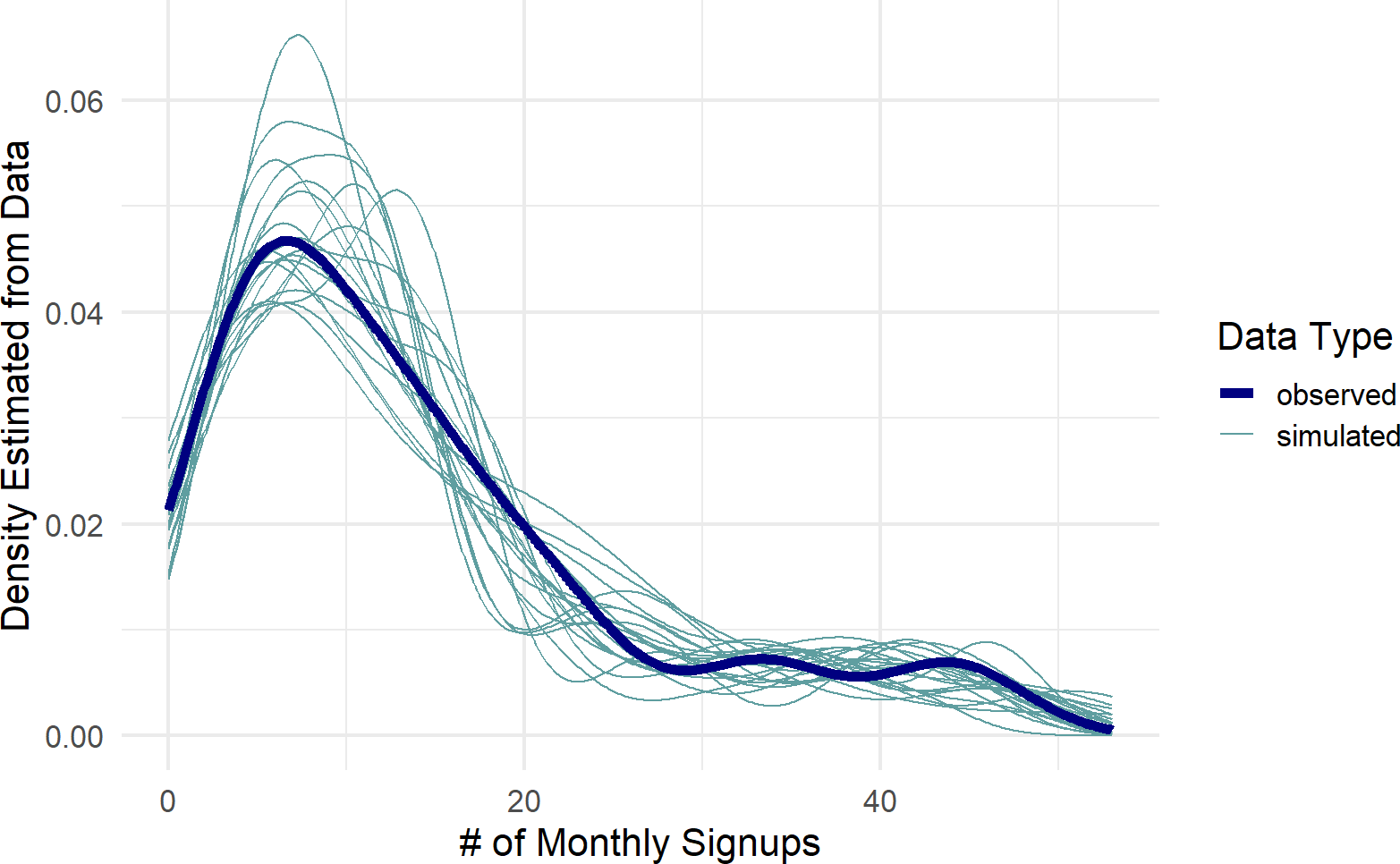
Figure 23.14 is encouraging!! It looks like the actual data might get generated from our posterior distribution. The partial pooling model seems to work! Hooray! Next chapter we interpret the results of this model for decision making.

23.5 Exercises

For this chapter’s exercises, we further examine the gymDF dataset of this chapter. Here is the model you should use to answer all exercises:

library(causact)
graph = dag_create() %>%
  dag_node("Number of Signups","k",
           rhs = binomial(nTrials,theta),
           data = gymDF$nSigned) %>%
  dag_node("Signup Probability","theta",
           child = "k",
           rhs = 1 / (1+exp(-y))) %>%
  dag_node("Number of Trials","nTrials",
           child = "k",
           data = gymDF$nTrialCustomers) %>%
  dag_node("Linear Predictor","y",
           rhs = alpha + beta * x,
           child = "theta") %>%
  dag_node("Yoga Stretch Flag","x",
           data = gymDF$yogaStretch,
           child = "y") %>%
  dag_node("Gym Intercept","alpha",
           rhs = normal(mu_alpha,sd_alpha),
           child = "y") %>%
  dag_node("Gym Yoga Slope Coeff","beta",
           rhs = normal(mu_beta,sd_beta),
           child = "y") %>%
  dag_node("Avg Crossfit Intercept","mu_alpha",
           rhs = normal(-1,1.5),
           child = "alpha") %>%
  dag_node("Avg Crossfit Yoga Slope","mu_beta",
           rhs = normal(0,0.75),
           child = "beta") %>%
  dag_node("SD Crossfit Intercept","sd_alpha",
           rhs = uniform(0,3),
           child = "alpha") %>%
  dag_node("SD Crossfit Yoga Slope","sd_beta",
           rhs = uniform(0,1.5),
           child = "beta") %>%
  dag_plate("Gym","j",
            nodeLabels = c("alpha","beta"),
            data = gymDF$gymID,
            addDataNode = TRUE) %>%
  dag_plate("Observation","i",
            nodeLabels = c("k","x","j",
                           "nTrials","theta","y"))
graph %>% dag_render()