Chapter 4 R: Basic Usage
4.1 Using the Console
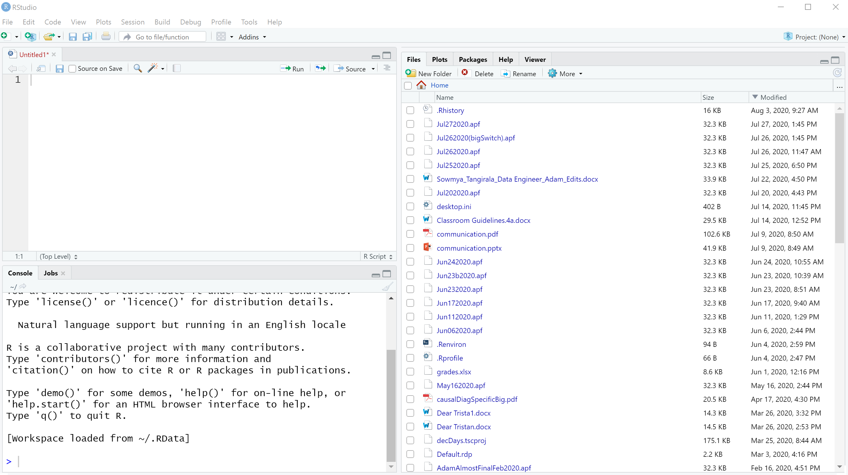
Open RStudio and start a new R-script by clicking the following menu options: File -> New File -> R Script. You should now see the four panes, a.k.a. windows, shown in Figure 4.1.
Figure 4.1: The RStudio user interface.
The easiest place to start using R is in bottom-left pane. This pane is known as the RStudio Console and acts very much like a calculator would. For example, type (2 + 1)^2 <ENTER> to square the result of 2+1:
## [1] 9Please notice that the order of operations is important. Here is the same code without the parentheses:
## [1] 3and you get a different result.
Tip: anytime you use parentheses, brackets, or braces, R will expect that there are closing parentheses, brackets, or braces for each one that is opened. A common experience is to forget to add the closing bracket. This causes the console’s \(>\) prompt for a command line to turn into a \(+\). For example, press <ENTER> after typing the following:
This yields no results. However, notice that the Console prompt has changed from a \(>\) symbol to a \(+\) symbol. This signals that the console is ready for more input. In this case, the lack of a closing parenthesis is a signal that more information should be coming. When this happens and you have no more input, you will want R to quit what it was doing and give back the > prompt. Click anywhere in the Console pane to set the focus of keyboard input on that pane and then, press <ESC> to return to the normal prompt. In theory, one can do all their work at the console’s command prompt, but this does not make for easy workflows. We will write in the upper-left pane, the Source Editor, for the majority of our coding.
4.2 Writing Scripts Using the Source Code Editor
While R can function as a calculator, we want to work with more than just one formula and one output at a time. In addition, we would like to be able to reproduce our results and modify our results with minimal effort. The top-left panel of RStudio (i.e. the Source Editor) facilitates this. Type the following in that pane using <ENTER> for line breaks:
You will notice nothing happens. If you want to run the above, called a script, then you must source the script by pressing the source button (Figure 4.2) in the pane’s upper-right hand corner and then seeing the code echoed with results in the Console.
 Figure 4.2: Source icon.
Alternatively, you can run any part of the code by selecting lines and pressing <CTRL>+<ENTER> (Mac users should use <CMD KEY>+<ENTER>). IMPORTANT NOTE FOR MAC USERS: Apple Mac users will use the command key in place of the control key. After running this script, you will notice that your environment panel (top-right of RStudio) now has values for a and b as shown in Figure 4.3.
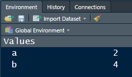 Figure 4.3: The Environment panel of RStudio showing that the object
 a is assigned the value of 2 and the object b is assigned the value of 4.
This panel reflects that object a is assigned the value of 2 and object b is assigned the value of 4.
4.3 Saving Scripts & Working Directories
You will notice that your three lines of code
are in a tab within the Source Editor pane titled Untitled1*. If you want to save this script for future use, you will want to click the save icon (Figure 4.4).
 Figure 4.4: Save icon.
As an alternative to the save icon, you can use the menus:
File -> Save.
This will bring up a dialog box requesting you to pick a file name and choose a save location. Create a new folder to store all of the files for this R session. Call this folder “Analytics” and place it in an easy to find location (e.g. C:/Analytics/). Save your script to that folder by naming the file myFirstScript.R and clicking Save. You can now reopen a saved script (File -> Open File) at any time to repeat your analysis.
Your working directory is the directory from which R will read and write files. One of the most common errors made by new users is to forget to set their working directory.4 When you are fed up with your file and directory organization, you should learn to associate one directory and one project. The Project capabilities in RStudio should be learned from here when you are ready: https://support.rstudio.com/hc/en-us/articles/200526207-Using-Projects. For now, try to remember to consciously read and write from a folder of your choosing. To set your working directory to your newly created C:/Analytics/ folder, use the RStudio menu sequence of Session -> Set Working Directory -> Choose Directory...
Figure 4.5: Using RStudio menus to choose your working directory.
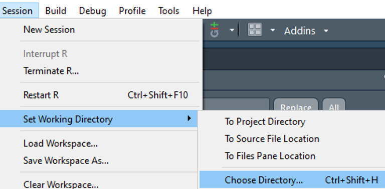
and select your C:/Analytics/ folder or whatever folder you created up above.
Create a new script and type the non-commented 5 Commented lines are not evaluated by the R programming language and are the lines beginning with #. Use these lines so that future you or other collaborators will more easily understand what your code is doing. lines below:
# A hash (i.e. #) on a line will comment out the rest
# of the line. You should heavily comment your scripts
# so that you and others can interpret them at a later
# time.  Comments are ignored by R.

# Reassign Values for a and b
a = 999
b = 111
a + b
## [1] 1110Instead of sourcing the script, let’s execute each line of the script individually.
Execute script lines individually by pressing
<CTRL> + <ENTER>.
To execute one line at a time, position your cursor on the line that says a = 999 and then press <CTRL> + <ENTER>. You will notice that your Environment tab in the upper-right pane now reflects the new value assigned to a (see Figure 4.6).
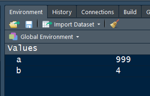 Figure 4.6: Updated environment values after overwriting the assigned value for
 a.
Use <CTRL> + <ENTER> two more times: 1) update the value for b and 2) calculate the sum of a and b.
Add the following (uncommented) lines to your script and then execute each of them individually:
# Source your first R-script to get back the original
# values.  Rememember that file names are case
# sensitive and to set your working directory to the
# location of the myFirstScript.R file.
source("myFirstScript.R")
a
b
a+b
## [1] 2
## [1] 4
## [1] 6This script illustrates the source function. The
source function in R executes code stored in a file. Notice
how the values of a and b are changed back to
the values assigned in myFirstScript.R.
Notice that your values for a and b have reverted back to the original values and their sum, a + b reflects the updated values. This is because myFirstScript.R contains code which is executed by the source("myFirstScript.R") line and overwrites the previous values.
4.4 R-objects: Scalars, Vectors, Dataframes, and Lists
In the previous section, you created two R-objects a and b. Single numbers assigned to variables like these are called scalars. The = sign was used to make the assignment, but using <- is an equally valid method of assigning value to an R-object.
As you progress though the material in this book. I encourage you to
create a new script for each chapter and write all of the shown code
into that script. You then use <CTRL>+<ENTER (PC)
or <CMD>+<ENTER> (Mac) to execute each line.
Save scripts with meaningful names and start new scripts anytime you
move to new work or a new chapter.
We will learn to create objects other than scalars, but before doing so, it makes sense to talk about naming objects. A syntactically valid name consists of letters, numbers and the dot (.) or underline (_) characters. Additionally, names must start with a letter or the dot not followed by a number. Names such as .2way are not valid, and neither are reserved words special to the R programming language (e.g. if else repeat while function for in next break TRUE FALSE). Additionally, please note the R is case-sensitive and even though it is possible, one should not name objects with commonly used R-functions (e.g. c sum mean source). Lastly, in terms of style, one should adopt one of the two more readily accepted naming conventions for variables:
- underscore separated: e.g. my_first_variable
- lowerCamelCase: e.g. myFirstVariable
My preference, and in this book, I will use lowerCamelCase.
4.4.1 Vectors
A vector is a sequence of data elements which all belong to the same type.6 The four basic data types for vectors are integer vectors, numerical vectors (i.e. numbers which may include non-integers), logical (i.e. TRUE or FALSE values), and character vectors (i.e. text). Further description for R’s data structures can be found at http://adv-r.had.co.nz/Data-structures.html. The concatenate function, c, can be used to create a vector:
You can do many things with vectors:
PRO TIP: Try using <Tab> after typing the first
few letters of an R-object. RStudio will often know how to
auto-complete the object’s name.
## [1] 4##Change the value of the third element
myFirstVector[3] = 10
##See the vector's content
myFirstVector## [1] 3 4 10 6## [1] 3 5 12 9## [1] 3 14 10 16## [1] 7 8 14 104.4.2 Matrices
A matrix is a 2-dimensional array where each element is of the same type (numeric/character/logical). There is a function called matrix that can be used to define a matrix:
We will not use matrices very often. Data frames, covered in the next section, represent a more common representation for data in data analysis.}
##      [,1] [,2]
## [1,]    7   14
## [2,] 8 10## [1] 14## [1] 8 10`matrix() is an example of a built-in function in R. A function is a set of code that automates a common task - in this case creating a matrix. Within the parantheses are arguments passed to the function - the inputs - and the function returns some useful output. We will learn more about functions in a few pages.
4.4.3 Data Frames
As business analysts, data frames are our favorite object in the R-ecosystem. We will use data frames to store data in rows and columns, just like a spreadsheet. When done right, columns will represent variables and rows represent observations. To illustrate this, we will use a built-in data frame that comes with R called mtcars. Make the data frame visible in your environment by running the following command:
carsDF object in it as shown in Figure 4.7.
Figure 4.7: The carsDF data frame is now shown in your global environment.
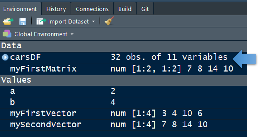
The expand icon (Figure 4.8) shown in the Environments pane will give an overview of the columns in the data frame. The spreadsheet icon (Figure 4.9) opens a tab to see the data in an easy to view form. To close this new tab, click the “x” next to the tab title (shown in Figure 4.10).
 Figure 4.8: Expand icon.
 Figure 4.9: Spreadsheet icon.
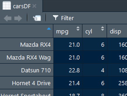 Figure 4.10: RStudio spreadsheet view of
 carsDF.
We can use this data frame to illustrate some useful ways of manipulating data frames:
# top line of data frame is called the header.
# the header is retrieved using the names function
names(carsDF)
## [1] "mpg" "cyl" "disp" "hp" "drat" "wt" "qsec" "vs" "am" "gear"
## [11] "carb"## [1] "Mazda RX4" "Mazda RX4 Wag" "Datsun 710"
## [4] "Hornet 4 Drive" "Hornet Sportabout" "Valiant"
## [7] "Duster 360" "Merc 240D" "Merc 230"
## [10] "Merc 280" "Merc 280C" "Merc 450SE"
## [13] "Merc 450SL" "Merc 450SLC" "Cadillac Fleetwood"
## [16] "Lincoln Continental" "Chrysler Imperial" "Fiat 128"
## [19] "Honda Civic" "Toyota Corolla" "Toyota Corona"
## [22] "Dodge Challenger" "AMC Javelin" "Camaro Z28"
## [25] "Pontiac Firebird" "Fiat X1-9" "Porsche 914-2"
## [28] "Lotus Europa" "Ford Pantera L" "Ferrari Dino"
## [31] "Maserati Bora" "Volvo 142E"## [1] 6## [1] 30.4# notice when you do not use quotes, R looks for
# an object instead of a value
carsDF["Honda Civic",mpg]# we can create objects to use as position references
gasMileage = c("mpg","hp")
carsDF["Honda Civic",gasMileage]## mpg hp
## Honda Civic 30.4 52Using <TAB> for auto-complete is a commonly used
shortcut in RStudio. This allows us to name R-objects very
descriptively without worrying about typing a million letters. For
example, instead of naming an object \(x\), be descriptive and name it something
useful, e.g. mythicalCreaturesDF for a list of fairy tale
creatures.
My favorite way to access a column of data is by using a winning combination of the $ operator and the <TAB> key. Try typing carsDF$ and then press <TAB>. You will see a list of all the columns in the carsDF data frame. Use the up and down arrows to pick the column you want to see and press <TAB> again to choose it. To make the auto-complete list smaller, you can type a letter contained within the column name. For example, typing carsDF$g and then pressing <TAB> limits the auto-complete list to the two columns where g is in the name: carsDF$gear and carsDF$mpg.
Once you select a column, this new object is no longer a data frame, it is a vector.
##  [1] 21.0 21.0 22.8 21.4 18.7 18.1 14.3 24.4 22.8 19.2 17.8 16.4 17.3 15.2 10.4
## [16] 10.4 14.7 32.4 30.4 33.9 21.5 15.5 15.2 13.3 19.2 27.3 26.0 30.4 15.8 19.7
## [31] 15.0 21.4
## return the first three elements of the vector
## the : is a shortcut to create a sequence of 1,2,3
carsDF$mpg[1:3]## [1] 21.0 21.0 22.84.4.4 Lists
A list is a vector of R-objects where the objects are not restricted to be the same type. The objects can be of any type and also, can be different lengths. There is a function called list that can be used to define a list:
x = 1   #a scalar
y = c(1,2) #a numeric vector
z = names(airquality) #a character(string) vector
df = mtcars  # a data frame

myFirstList = list(x,y,z,df)

# slice the list using single brackets
# (the results of doing this returns a list)
myFirstList[3]
## [[1]]
## [1] "Ozone" "Solar.R" "Wind" "Temp" "Month" "Day"# use double brackets to reference a member directly
# (this returns a character vector)
myFirstList[[3]]## [1] "Ozone" "Solar.R" "Wind" "Temp" "Month" "Day"4.5 Functions
Functions are sets of instructions intended to perform a specific set of actions. They are used to minimize typing for a set of instructions that are to be used repeatedly and to create more readable code by hiding code complexity which distracts from the essence of a program. A function accepts arguments or parameters as input and it will return one or more values. To create a user-defined function, we need to create a function that conforms to this basic construct:
Functions and their arguments can be named just like any other
R-object. So myFirstFun and
myFirstArgument could have been named differently, I chose
those names to be descriptive.
Once the definition of the function is entered into the environment, we can call the function from other parts of the code, i.e. we can use it. The following code defines a function that computes the square of the argument and then calls it after assigning a value for its argument:
# define a simple function with one argument called
# myFirstArgument.  note: myFirstFun is just another
# R-object.  In this case, it is a function.
myFirstFun = function(myFirstArgument)
{
  #  compute the square, assign it to object z
  z = myFirstArgument * myFirstArgument
  return(z) #function returns the squared value
}

# call the function with a number you wish to square
m = myFirstFun(myFirstArgument = 8)
m # print the value
## [1] 64# you can exclude the argument name if you supply the
# argument values in the order the function expects
myFirstFun(9)## [1] 81Multiple arguments are also possible. The following is a two-argument function called adamSumsSquares which takes two arguments, squares each argument, and then returns their sum.
Exercise 4.1 Create a new function called squareSumOfThreeNumbers which takes three arguments arg1, arg2, and arg3. The function should add three numbers together and then square the sum. Write the code for the new function and then test that code by computing the following:
So far, you have seen a variety of functions such as source, data.frame, matrix, and list. Throughout the book, you will learn many more functions that help us to get our work done more effectively. If you have questions about how to use a function, the help function can show you example usage as shown here:
Also, ChatGPT, Google and YouTube searches should be relied on heavily. Even expert programmers regularly use these searches. Part of the learning process and the pain of becoming fluent in coding is to become better at using search terms that yield results for your particular problem.
4.6 Exercises
Exercise 4.2 Without running the below code, predict the output (i.e. the value of x).
Verify your answer by creating a new script with the above code.
Exercise 4.3 Create a new data frame object called airQualityDF by assigning it the value of a built-in dataset called airquality. Use R-code to reference the cell value that contains the temperature of the \(15^{th}\) observation.
Exercise 4.4 Enter these two lines into the Console Window of RStudio (lower left hand window):
The object “x” is now assigned a random value between 1 and 50. You can simply type x followed by ENTER and you will be able to see its value. Now, combine the numbers 4,5,8, & 11, along with the object x, into a vector using the following R code:
The vector will have five numbers. Now use the sum function to return the sum of the elements in b. What is the value of that sum?
Exercise 4.5 Sometimes, you will find it useful to create your own function. At its core, a function takes arguments and returns an interesting result. For example, I can create a two-argument function called adamSumsSquares which takes two arguments, squares each argument, and then returns their sum. The code for this would be:
I can then use this function by writing:
which returns a result of 52.
Create a function called squareSums. This function should accept three arguments, sum them up, and then square the sum. Verify your function works by running:
To know you did this right, the above command must return a result of 202.