Chapter 10 Representing Uncertainty
Real-world uncertainty makes decision making hard. Conversely, without uncertainty decisions would be easier. For example, if a cafe knew exactly 10 customers would want a bagel, then they could make exactly 10 bagels in the morning; if a factory’s machine could make each part exactly the same, then quality control to ensure the part’s fit could be eliminated; if a customer’s future ability to pay back a loan was known, then a bank’s decision to underwrite the loan would be quite simple.
In this chapter, we learn to represent our real-world uncertainty (e.g. demand for bagels, quality of a manufacturing process , or risk of loan default) in mathematical and computational terms. We start by defining the ideal mathematical way of representing uncertainty, namely by assigning a probability distribution to a random variable. Subsequently, we learn to describe our uncertainty in a random variable using representative samples as a pragmatic computational proxy to this mathematical ideal.
10.1 Random Variables With Assigned Probability Distributions
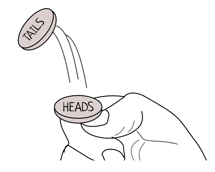 Figure 10.1: The outcome of a coin flip can be represented by a probability distribution.
Think of a random variable as a mapping from potential outcomes to numerical values representing the probability we assign to each outcome. For us business folk, we can often think of this mapping as a table with outcomes on the left and probabilities on the right; take this table of coin flip outcomes as an example:
Table 10.1: Using a table to represent the probability distribution of a coin flip.
| Outcome | Probability |
|---|---|
| HEADS | 50% |
| TAILS | 50% |
While Table 10.1 might be adequate to describe the mapping of coin flip outcomes to probability, as we make more complex models of the real-world, we will want to take advantage of the concise (and often terse) notation that mathematicians would use. In addition, we want to gain fluency in math world notation so that we can successfully traverse the bridge between real world and math world. Random variables are the fundamental math world representation that create the foundation of our studies, so please resist any temptation to not learn the subsequent mathematical notation.
10.1.1 Some Math Notation for Random Variables
Mathematicians love using Greek letters, please do not be intimidated by them - they are just letters. You will learn lots of lowercase letters like \(\alpha\) (alpha), \(\beta\) (beta), \(\mu\) (mu), \(\omega\) (omega), and \(\sigma\) (sigma). And also some of their uppercase versions like \(\Omega\) (omega) as the uppercase of \(\omega\). See the whole list at wikipedia.org.
Above, a random variable was introduced as a mapping of outcomes to probabilities. And, this is how you should think of it most of the time. However, to start gaining fluency in the math-world definition of a random variable, we will also view this mapping process as not just one mapping, but rather a sequence of two mappings: 1) the first mapping is actually the “true” probability-theory definition of a random variable - it maps all possible outcomes to real numbers, and 2) the second mapping, known as a probability distribution in probability theory, maps the numbers from the first mapping to real numbers representing how plausibility is allocated across all possible outcomes - we often think of this allocation as assigning probability to each outcome.
For example, to define a coin flip as a random variable Please note that the full mathematical formalism of random variables is not discussed here. For applied problems, thinking of a random variable as representing a space of possible outcomes governed by a probability distribution is more than sufficient., start by listing the set of possible outcomes (by convention, the greek letter \(\Omega\) is often used to represent this set and it is called the sample space): \[\Omega = \{Heads,Tails\}.\] The outcomes in a sample space must be 1) exhaustive i.e. include all possible outcomes and 2) mutually exclusive i.e. non-overlapping. Then pick an an uppercase letter, like \(X\), to represent the random variable (i.e. an unobserved sample from \(\Omega\)) and explictly state what it represents using a short description: \[X \equiv \textrm{The outcome of a coin flip,}\] where \(\equiv\) is read “defined as”.
When real-world outcomes are not interpretable real numbers (e.g. heads and tails), define an explicit mapping of these outcomes to real numbers:
\[ X \equiv \begin{cases} 0, & \textrm{if outcome is } Tails \\ 1, & \textrm{if outcome is } Heads \end{cases} \]
For, coin flip examples, it is customary to map heads to the number 1 and tails to the number 0. Thus, \(X=0\) is a concise way of saying “the coin lands on tails” and likewise \(X=1\) means “the coin lands on heads”. The terse math-world representation of a mapping process like this is denoted:
Mathematicians use the symbol \(\mathbb{R}\) to represent the set of all real numbers.
\[X:\Omega \rightarrow \mathbb{R}\], where you interpret it as “random variable \(X\) maps each possible outcome in sample space omega to a real number.”
The second mapping process then assigns a probability distribution to the random variable. By convention, lowercase letters, e.g. \(x\), represent actual observed outcomes. We call \(x\) the realization of random variable \(X\) and define the mapping of outcomes to probability for every \(x \in X\) (read as \(x\) “in” \(X\) and interpret it to mean “for each possible realization of random variable \(X\)”). As you would already guess, we have 100% confidence that one of the outcomes will be realized (e.g. heads or tails), so as such and by convention, we allocate 100% plausibility (or probability) among the possible outcomes. In this book, we will use \(f\), to denote a function that maps each possible realization of a random variable to its corresponding plausibilty measure and use a subscript to disambiguate which random variable is being referred to when necessary. For the coin flip example, we can use our newly learned mapping notation to demonstrate this:
There are several conventions for representing this mapping function which takes a potential realization as input and provides a plausibility measure as output. This textbook uses all of them. Right now, you see \(f_X(x)\) or more simply just \(f(x)\), but other equally valid notation will use \(\pi(x)\), \(Pr(X=x)\), or \(p(x)\). Knowing that there is not just one standard convention will prove useful as you read other texts about probability. After a while, this change of notation becomess less frustrating.
\[f_X: X \rightarrow [0,1],\] where \([0,1]\) is notation for a number on the interval from 0 to 1; the square brackets mean the interval is closed and hence, the mapping of an outcome to exactly 0 or 1 is possible.
Despite all this fancy notation, for small problems it is sometimes the best course of action to think of a random variable as a lookup table as shown here:
Table 10.2: Probability distribution for random variable \(X\) represented as a table showing how real-world outcomes are mapped to real numbers and how 100% plausibility is allocated between all of the outcomes.
| Outcome | Realization (\(x\)) | \(f(x)\) |
|---|---|---|
| HEADS | 1 | 0.5 |
| TAILS | 0 | 0.5 |
and where \(f(x)\) can be interpreted as the plausability assigned to random variable \(X\) taking on the value \(x\). For example, \(f(1) = 0.5\) means that \(Pr(X=1) = 50\%\) or equivalently that the probability of heads is 50%.
To reiterate how a random variable is a sequence of two mapping processes, notice that Table 2.2 has these features:
- It defines a mapping from each real-world outcome to a real number.
- It allocates plausibility (or probability) to each possible realization such that we are 100% certain one of the listed outcomes will occur.
10.1.2 The Power of Abstraction
“[We will] dive deeply into small pools of information in order to explore and experience the operating principles of whatever we are learning. Once we grasp the essence of our subject through focused study of core principles, we can build on nuanced insights and, eventually, see a much bigger picture. The essence of this approach is to study the micro in order to learn what makes the macro tick.” - Josh Waitzkin
While the coin flip example may seem trivial, we are going to take that micro-example and abstract a little bit. As Josh Waitzkin advocates (Waitzkin 2007Waitzkin, Josh. 2007. The Art of Learning: A Journey in the Pursuit of Excellence. Simon; Schuster.), we should “learn the macro from the micro.” In other words, master the simple before moving to the complex. Following this guiding principle, we will now make things ever-so-slightly more complex. Let’s model uncertain outcomes where there are two possibilities - like a coin flip, but now we assume the assigned probabilities do not have to be 50%/50%. Somewhat surprisingly, this small abstraction now places an enormous amount of real-world outcomes within our math-world modelling capabilities:
 Figure 10.2: Ars Conjectandl - Jacob Bernoulli’s post-humously published book (1713) included the work after which the notable probability distribution - the Bernoulli distribution - was named.
- Will the user click my ad?
- Will the drug lower a patient’s cholesterol?
- Will the new store layout increase sales?
- Will the well yield oil?
- Will the customer pay back their loan?
- Will the passenger show up for their flight?
- Is this credit card transaction fraudulent?
The Bernoulli distribution, introduced in 1713 (see Figure 10.2), is a probability distribution used for random variables of the following form:
Table 10.3: If \(X\) follows a Bernoulli distribution, then the following lookup table describes the mapping process.
| Outcome | Realization (\(x\)) | \(f(x)\) |
|---|---|---|
| Failure | 0 | \(1-p\) |
| Success | 1 | \(p\) |
In Table (ref?)(tab:bern), \(p\) is called a parameter of the Bernoulli distribution. Given the parameter(s) of any probability distribution, you can say everything there is to know about a random variable following that distribution; this includes the ability to know all possible outcomes as well as their likelihood. For example, if \(X\) follows a Bernoulli distribution with \(p=0.25\), then you know that \(X\) can take the value of 0 or 1, that \(Pr(X=0) = 0.75\), and lastly that \(Pr(X=1) = 0.25\)
where \(p\) represents the probability of success - notice that the following must hold to avoid non-sensical probability allocations \(0 \leq p \leq 1\).
With all of this background, we are now equipped to model uncertainty in any observable data that has two outcomes. The way we will represent this uncertainty is using two forms: 1) a graphical model and 2) a statistical model. The graphical model is simply an oval - yes, we will draw random variables as ovals because ovals are not scary, even to people who don’t like math:
Figure 10.3: This oval represents a random variable indicating the result of a coin flip.
And, the statistical model is represented using \(\equiv\) to provide a real-world definition of our random variable and \(\sim\) to assign a probability distribution:
\[ \begin{aligned} X &\equiv \textrm{Coin flip outcome with heads}=1 \textrm{ and tails}=0.\\ X &\sim \textrm{Bernoulli}(p) \end{aligned} \]
\(\sim\) is read “is distributed”; so you say “X is distributed Bernoulli with parameter \(p\).”
We will see in future chapters that the graphical model and statistical models are more intimately linked than is shown here, but for now, suffice to say that the graphical model is good for communicating uncertainty to stakeholders more grounded in the real-world and the statistical model is better for communicating with stakeholders in the math-world.
10.2 Representative Samples
Despite our ability to represent probability distributions using precise mathematics, uncertainty modelling in the practical world is always an approximation. Does a coin truly land on heads 50% of the time (see https://en.wikipedia.org/wiki/Checking_whether_a_coin_is_fair)? It is hard to tell. One might ask, how many times must we flip a coin to be sure? The answer might surprise you; it could take over 1 million tosses to reach an estimate that a coin lies within 0.1% of the observed proportion of heads. That is a lot of tosses. So in the real world, seeking that level of accuracy becomes impractical. Rather, we are seeking a model that is good enough; a model where we believe in its insights and are willing to follow through with its recommendations.
A representative sample is an incomplete collection or subset of data that exhibits a specific type of similarity to a complete collection of data from an entire (possibly infinite) population. For our purposes, the similarity criteria requires that an outcome drawn from either the sample or the population is drawn with similar probability.
Instead of working with probability distributions directly as mathematical objects, we will most often seek a representative sample and treat them as computational objects (i.e. data). For modelling a coin flip, the representative sample might simply be a list of \(heads\) and \(tails\) generated by someone flipping a coin or by a computer simulating someone flipping a coin.
Turning a mathematical object into a representative sample using R is quite easy as R (and available packages) can be used to generate random outcomes from just about all well-known probability distributions. To generate samples from a random Bernoulli variable, we use the rbern function from the causact package:
# The rbern function is in the causact package
library(causact)
# rbern is a function that takes two arguments:
# 1) n is the number of trials (aka coin flips)
# 2) prob is the probability of success (aka the coin lands on heads)
set.seed(123)
rbern(n=7,prob=0.5)
## [1] 0 1 0 1 1 0 1The set.seed() function takes an integer argument. If
your computer and my computer supply the same integer argument to this
function (e.g. 123), then we will get the same random
numbers even though we are on different computers. I use this function
when I want your “random” results and my “random” results to match
exactly.
where the 3 0’s and 4 1’s are the result of the n=7 coin flips.
Notice that one might be reluctant to label this a representative sample as the proportion of 1’s is 0.57 and not the 0.5 that a representative sample would be designed to mimic. In fact, we can write code to visualize the proportion of heads as a function of the number of coin flips:
library(tidyverse)
set.seed(123)

# Create dataframe of coinflip observations
numFlips = 50 ## flip the coin 50 times
df = data.frame(
  flipNum = 1:numFlips,
  coinFlip = rbern(n=numFlips,prob=0.5)
  ) %>%
  mutate(headsProportion = cummean(coinFlip))

# Plot results
ggplot(df, aes(x = flipNum, y = headsProportion)) +
  geom_point() +
  geom_line() +
  geom_hline(yintercept = 0.5, color = "red") +
  ggtitle("Running Proportion of Heads") +
  xlab("Flip Number") +
  ylab("Proportion of Heads") +
  ylim(c(0,1))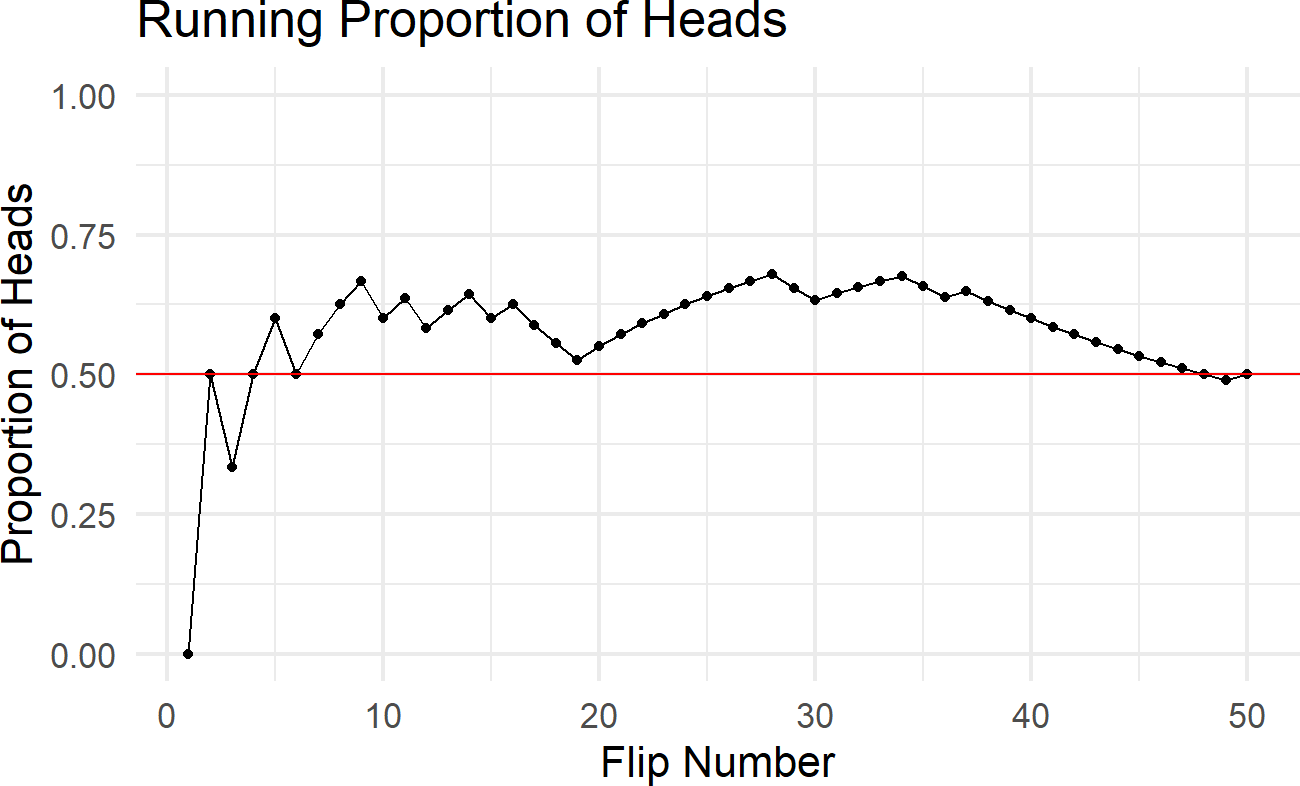
Notice that even after 30 coin flips, the sample is far from representative as the proportion of heads is 0.63. Even after 1,000 coin flips (i.e. numFlips = 1000), the proportion of heads 0.493 is still just an approximation as it is not exactly 0.5.
Well if 1,000 coin flips gets us an approximation close to 0.5, then 10,000 coin flips should get us even closer. To explore this idea, we generate ten simulations of 10,000 coin flips and print out the average proportion of heads for each:
set.seed(123)
for (i in 1:10){
  proportionOfHeads =
    mean(rbern(n=10000,prob=0.5))
  print(proportionOfHeads)
}
## [1] 0.4943
## [1] 0.4902
## [1] 0.4975
## [1] 0.4888
## [1] 0.4997
## [1] 0.5006
## [1] 0.4954
## [1] 0.4982
## [1] 0.5083
## [1] 0.5011Notice that the average distance away from the exact proportion 0.5 is 0.459%. So on average, it appears we are around 0.5% away from the true value. This is the reality of representative samples; they will prove enormously useful, but are still just approximations of the underlying mathematical object - in this case, \(X \sim \textrm{Bernoulli}(0.5)\). If this approximation bothers you, remember the mathematical object is just an approximation of the real-world object. Might it be possible that certain coins are weighted in one way or another to deviate - even ever so slightly - from the ideal? Of course, but it does not mean the approximations are useless … on the contrary, we will see how powerful the math-world and computation-world can be in bringing real-world insight.
10.2.1 Generating representative samples
So far, we have represented uncertainty in a simple coin flip - just one random variable. As we try to model more complex aspects of the business world, we will seek to understand relationships between random variables (e.g. price and demand for oil). Starting with our simple building block of drawing an oval to represent one random variable, we will now draw multiple ovals to represent multiple random variables. Let’s look at an example with more than one random variable:
Example 10.1 The XYZ Airlines company owns the one plane shown in Figure 10.4. XYZ operates a 3-seater airplane to show tourists the Great Barrier Reef in Cairns, Australia. The company uses a reservation system, wherein tourists call in advance and make a reservation for aerial viewing the following day. Unfortunately, often passengers holding a reservation might not show up for their flight. Assume that the probability of each passenger not showing up for a flight is 15% and that each passenger’s arrival probability is independent of the other passengers. Assuming XYZ takes three reservations, use your ability to simulate the Bernoulli distribution to estimate a random variable representing the number of passengers that show up for the flight.
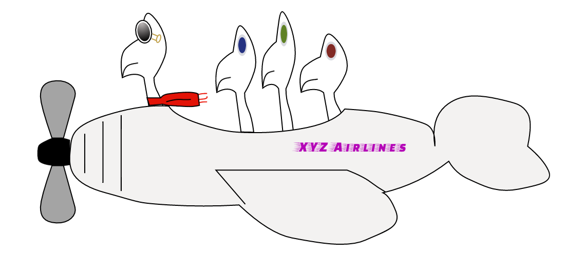 Figure 10.4: How many passengers will show up if XYZ Airlines accepts three reservations.
To solve Example 10.1, we take the real-world problem and represent it mathematically with three random variables: 1) \(X_1 \equiv\) whether passenger 1 shows up, 2) \(X_2 \equiv\) whether passenger 2 shows up, and 3) \(X_3 \equiv\) whether passenger 3 shows up. And to answer the question of how many passengers show up, we define one more random variable, \(Y = X_1 + X_2 + X_3\). Since \(Y\) is a function of the other three random variables, we will use arrows in our graphical model to indicate this relationship:
Figure 10.5: The graphical model of number of passengers who show up for the XYZ airlines tour.
And, the statistical model is represented like this:
\[ \begin{aligned} X_i &\equiv \textrm{If passenger } i \textrm{ shows up, then } X=1 \textrm{. Otherwise, } X = 0 \textrm{. Note: } i \in \{1,2,3\}.\\ X_i &\sim \textrm{Bernoulli}(p = 0.85)\\ Y &\equiv \textrm{Total number of passengers that show up.}\\ Y &= X_1 + X_2 + X_3 \end{aligned} \]
The last line gives us a path to generate a representative sample of the number of passengers who show up for the flight; we simulate three Bernoulli trials and add up the result. Computationally, we can create a data frame to simulate as many flights as we want. Let’s simulate 1,000 flights and see the probabilities associated with \(Y\):
library(causact)
numFlights = 1000 ## number of simulated flights
probShow = 0.85 ## probability of passenger showing up

# choose random seed so others can
# replicate results
set.seed(111)

pass1 = rbern(n = numFlights, prob = probShow)
pass2 = rbern(n = numFlights, prob = probShow)
pass3 = rbern(n = numFlights, prob = probShow)

# create data frame (use tibble to from tidyverse)
flightDF = tibble(
  simNum = 1:numFlights,
  totalPassengers = pass1 + pass2 + pass3
)

# transform data to give proportion
propDF = flightDF %>%
  group_by(totalPassengers) %>%
  summarize(numObserved = n()) %>%
  mutate(proportion = numObserved / sum(numObserved))

# plot data with estimates
ggplot(propDF,
       aes(x = totalPassengers, y = proportion)) +
  geom_col() +
  geom_text(aes(label = proportion), nudge_y = 0.03)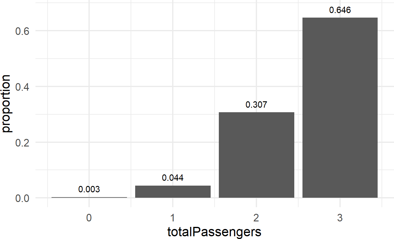
Wow, that was pretty cool. We created a representative sample for a random variable whose distribution was not Bernoulli, but could be constructed as the sum of three Bernoulli random variables. We can now answer questions like “what is the probability there is at least one empty seat?” This is the same as saying what is \(Pr(Y<=2)\) or equivalently \(1 - Pr(Y=3)\). And the answer, albeit an approximate answer, is 0.354.
You may be wondering how much the approximated probabilities for the
number of passengers might vary with a different simulation. The best
way to find out is to try it again. Remember to eliminate or change the
set.seed function prior to trying the simulation again.
10.3 Mathematics As A Simulation Shortcut
Simulation will always be your friend in the sense that if given enough time, a simulation will always give you results that approximate mathematical exactness. The only problem with this friend is it is sometimes slow to yield representative results. In these cases, sometimes mathematics provides a shortcut. The shortcut we study here is to define a probability distibution.
10.3.1 Probability Distributions and Their Parameters
One cool math shortcut is to use named probability distributions. Each named distribution (e.g. Bernoulli, normal, uniform, etc.) has a set of parameters (i.e. values provided by you) that once specified tell you everything there is to know about a random variable - let’s call it \(X\). Previously, we learned that \(p\) is the one parameter of a Bernoulli distribution and it can be used to describe \(X\) as such:
\[ \textrm{Bernoulli}(p) \]
Once we give \(p\) a value, say \(p=0.4\), then we know everything there is to know about random variable \(X\). Specifically, we know its possible values (i.e. 0 or 1) and we know the probability of those values:
| Realization (\(x\)) | \(f(x)\) |
|---|---|
| 0 | \(60\%\) |
| 1 | \(40\%\) |
This is the shortcut. Once you name a distribution and supply its parameters, then its potential values and their likelihood are fully specified.
10.3.2 The Binomial Distribution
The two parameters of a binomial distribution map to the real-world in a fairly intuitive manner. The first parameter, \(n\), is simply the number of Bernoulli trials your random variable will model. The second parameter, \(p\), is the probability of observing success on each trial. So if \(X \equiv \textrm{number of heads in 10 coin tosses}\) and \(X \sim \textrm{Binomial}(n=10, p=0.5)\), then an outcome of \(x=4\) means that four heads were observed in 10 coin flips.
A particularly useful two-parameter distribution was derived as a generalization of a Bernoulli distribution. None other than Jacob Bernoulli himself realized that just one Bernoulli trial is sort of uninteresting (would you predict the next president by polling just one person?). Hence, he created the binomial distribution.
The binomial distribution is a two-parameter distribution. You specify the values for the two parameters and then, you know everything there is to know about a random variable which is binomially distributed. The distribution models scenarios where we are interested in the cumulative outcome of successive Bernoulli trials - something like the number of heads in multiple coin flips or the number of passengers that arrive given three reservations. More formally, a binomial distributed random variable (let’s call it \(X\)) represents the number of successes in \(n\) Bernoulli trials where each trial has success probability \(p\). \(n\) and \(p\) are the two-parameters that need to be specified.
Going back to our airplane example (Example 10.1), we can take advantage of the mathematical shortcut provided by the binomial distribution and use the following graphical/statistical model combination to yield exact results. The graphical model is just a simple oval:
Figure 10.6: The graphical model of number of passengers who show up for the XYZ airlines tour.
And, the statistical model is represented like this:
\[ \begin{aligned} Y &\equiv \textrm{Total number of passengers that show up.}\\ Y &\sim \textrm{Binomial}(n = 3, p = 0.85) \end{aligned} \]
For just about any named probability distribution, like the binomial distribution, R can be used to both answer questions about the probability of certain values being realized, as well as, to generate random realizations of a random variable following that distribution. We just need to know the right function to use. Thanks to an established convention, functions for probability distributions in R mostly adhere to the following syntax:
foo is called a placeholder name in computer
programming. The word foo itself is meaningless, but you
will substitute more meaningful words in its place. In the examples
here, foo will be replaced by an abrreviated probability
distribution name like binom or norm.
dfoo()- is the probability mass function or the probability density function (PDF). For discrete random variables, the PDF is \(Pr(X=x)\). A user inputs \(x\) and parameters of \(X\)’s distribution, the function returns \(Pr(X=x)\). For continuous random variables, this number is less interpretable (see this Khan Academy video for more background information). Typical math notation for this function is \(f(x)\).pfoo()- is the cumulative distribution function (CDF). User inputs \(q\) and specifies parameters of the distribution, the CDF returns a probability \(p\) such that \(Pr(X \leq q)=p\). Typical math notation for this function is \(F(q)\).qfoo()- is the quantile function. User inputs \(p\) and parameters of the distribution, this returns the realization value \(q\) such that \(Pr(X \leq q) = p\). Corresponding math notation for this function is \(F^{-1}(p)\).rfoo()- is the random generation function. User inputs \(n\) and the distribution parameters, this returns \(n\) random observations of the random variable.
Take notice of the transformatiion from the math world to the
computation world. In the math world, we might say \(Y \sim \textrm{Binomial}(n=3,p=0.85)\). But
in the computation world of R, \(n\) is
replaced by the size argument and \(p\) is replaced by the prob
argument. Also notice that n is an argument of the
rfoo function, but it is not the same as the math-world
\(n\). In the computer-world
n is the number of random observations of a specified
distribution that you want generated. So if you wanted 10 samples of
\(Y\), you would use the function
rbinom(n=10,size=3,prob=0.85). Be careful when doing these
translations.
Since we are interested in the binomial distribution, we can replace foo by binom to take advantage of the probability distribution functions listed above. For example, to answer “what is the probability there is at least one empty seat?” We find \(1 - Pr(Y=3)\) which is the same as 1 - dbinom(x=3, size = 3, prob = 0.85). And the exact answer is 0.385875. Note, this is very close, but not identical, to our previously approximated answer of 0.354. We could have chosen to use the CDF instead of the PDF to answer this question by finding \(Pr(Y \leq 2)\) using pbinom(q=2, size = 3, prob = 0.85). To reproduce our approximated results using the exact distribution, we can use the following code:
# transform data to give proportion
propExactDF = tibble(totalPassengers = 0:3) %>%
  mutate(proportion =
           dbinom(x = totalPassengers,
                  size = 3,
                  prob = 0.85))

# plot data with estimates
ggplot(propExactDF, aes(x = totalPassengers,
                        y = proportion)) +
  geom_col() +
  geom_text(aes(label = proportion),
            nudge_y = 0.03)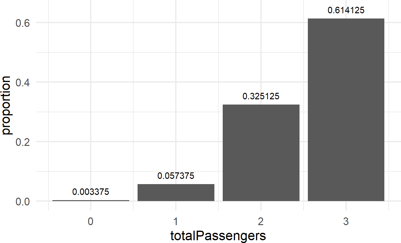
The above code is both simpler and faster than the approximation code run earlier. In addition, it gives exact results. Hence, when we can take mathematical shortcuts, we will to save time and reduce the uncertainty in our results introduced by approximation error.
10.4 Big Picture Takeaways
This chapter is our first foray into representing uncertainty. Our representation of uncertainty takes place in three worlds: 1) the real-world - we use graphical models (i.e. ovals) to convey the story of uncertainty, 2) the math-world - we use statistical models to rigorously define how random outcomes are generated, and 3) the computation-world - we use R functions to answer questions about exact distributions and representative samples to answer questions when the exact distribution is unobtainable. As we navigate this course, we will traverse across these worlds and learn to translate from one world’s representation of uncertainty to another’s.
10.5 Getting Help
Google and YouTube are great resources to supplement, reenforce, or further explore topics covered in this book. For the mathematical notation and conventions regarding random variables, I highly recommend listening to Sal Khan, founder of Khan Academy, for a more thorough introduction/review of these concepts. Sal’s videos can be found at https://www.khanacademy.org/math/statistics-probability/random-variables-stats-library.
10.6 Exercises
Exercise 10.1 Assume you want to use the rnorm function in R to create a representative sample of a random variable that is
normally distributed with mean 0 and standard deviation of 5000.
Execute set.seed(444) immediately prior to generating a 1,000 element representative sample for this random variable. You will notice that the mean of this sample is not quite equal to zero. Report the mean for this sample (rounded to three decimal places) and comment why it is not zero.
Exercise 10.2 Often, I want you to be able to find information on the internet that aids your ability to accomplish your analytics goals. In this question, assume you want to generate a continous uniform distribution in R using one of the rfoo functions (i.e. rnorm, rtruncnorm). (note: The use of the word foo in computer science is explained here: https://en.wikipedia.org/wiki/Metasyntactic_variableLinks to an external site.). Find the R function (in the form rfoo) that can generate n uniform random numbers that lie in the interval (min, max) to create a representative sample of a random variable that is uniformly distributed between 0 and 100.
Execute set.seed(111) immediately prior to generating a 2000-element representative sample for this random variable. Report the maximum number below (rounded to three decimal places).
Exercise 10.3 An expert on process control states that he is 95% confident that the new production process will save between $6 and $9 per unit with savings values around $7.50 more likely. If you were to model this expert’s opinion using a normal distribution (i.e. google “empirical rule for normal distribution”), what standard deviation would you use for your normal distribution?
Exercise 10.4 Use dbinom to answer this question: A shop receives a batch of 1,000 cheap lamps. The odds that a lamp are defective are 0.4%. Let X be the number of defective lamps in the batch. What is the probability the batch contains exactly 2 defective lamps (i.e. X=2)? Report as decimal with three significant digits.
Exercise 10.5 Use pbinom to answer this question: A shop receives a batch of 1,000 cheap lamps. The odds that a lamp are defective are 0.4%. Let X be the number of defective lamps in the batch. What is the probability the batch contains less than or equal to 2 defective lamps (i.e. \(X \leq 2\))? Report as decimal with three significant digits.