Chapter 17 The beta Distribution
Figure 17.1: Our typical generative model for Bernoulli data. In this chapter, we will move away from using a uniform distribution and explore the beta distribution as a prior distribution for theta.
Making a model requires constructing a set of inter-related random variables. Some of these random variables are observed and others are latent (i.e. nto observed). A common pattern is to:
- Assume observed data comes from a specified family of probability distributions. So far, that known family has been the
Bernoullidistribution. - Use latent variables to model uncertainty in the parameters of the distribution family in step 1. So far, this uncertainty was modeled with the uniform distribution.
Note the subtle difference in how probability distributions are used to model observed versus latent/unobserved variables. When observed random variables are modelled, it is to establish the likelihood component of Bayes theorem, i.e. \(P(Data|Model)\). When latent random variables are modelled, it is to establish the prior allocation of plausibility over all possible values, i.e. \(P(Model)\). Two important and contrasting implications regarding the generative model implied by a posterior distribution are: 1) the posterior recipe is restricted to modelling observed data as generated from the specified distribution, and 2) the posterior recipe is not restricted to a specific distribution when modelling uncertainty in latent variables. This tricky difference will be explored in this chapter, but if this is your first read-through, just remember that distributions modelling prior uncertainty do NOT imply that posterior uncertainty will also be from the same distribution.
Figure 17.1 is the generative DAG we have been working with to date. It contains two inter-related random variables \(X\) and \(\Theta\). For any observed realization \(x\), we assume it came from a \(\textrm{Bernoulli}(\theta)\) generating process; i.e. there is zero uncertainty that the data is generated from a \(\textrm{Bernoulli}\) distribution. Given a specified \(\theta\), the uncertainty in \(X\) is purely due to the stochastic nature of a Bernoulli random variable. The takeaway is that for observed data, our statistical model restricts the generative recipe to be from the specified family - i.e. Bernoulli.
We also model uncertainty in the unobserved random variable \(\Theta\). Modelling uncertainty in unobserved RV’s is different in that the posterior distribution of \(\theta\) is not restricted to be from the same distribution family as its prior specification. In fact, for most cases our posterior distribution for unobserved random variables cannot be summarized using a known distribution family (e.g. normal, uniform, etc.); posteriors will only be approximated with representative samples as that is the best we can do.
When it comes to representing prior uncertainty, try to pick a distribution whose support The support of a random variable and its associated probability distribution is the set of possible realizations with non-zero probability density. covers all possible realizations of the RV. For \(\Theta\), this would be a probability distribution whose support is all values such that \(0 \leq \theta \leq 1\). The \(\textrm{Uniform}(0,1)\) distribution provided an example where prior uncertainty mapped to all possible values of \(\theta\), but after updating that uncertainty in light of data, we have already seen that the posterior distribution was no longer uniform.
The takeaway is that for unobserved data, our generative DAG contributes a prior, but the posterior for that RV is not restricted to be from the specified family. For example, the posterior for \(\theta\) will not be uniformly distributed despite having a uniform prior.
If we do not have uniform beliefs about plausible values for \(\theta\), there is another well-known and more-flexible distribution that can be used as a prior for \(\theta\). In other words, if you were to ask a statistician “what other distributions have support that ensures \(0 \leq \theta \leq 1\)?”, a likely response you will get is the \(\textrm{beta}\) distribution. In the absence of a statistician, go to wikipedia, https://en.wikipedia.org/wiki/List_of_probability_distributions, and find a useful list of probability distributions. You’ll see the first one in the list is the Bernoulli distribution. To find others that might be useful in a certain case:
- Match the support of the distribution with what you think is feasible. The wikipedia list has multiple categories for support, we have only seen these two so far:
- Discrete with finite support (e.g. Bernoulli)
- Continuous on a bounded interval (e.g. uniform)
- Investigate how changing parameters can make a distribution more consistent with the assumptions you are willing to make about your generative recipe.
The wikipedia entry, https://en.wikipedia.org/wiki/Beta_distribution, for the beta distribution is where a statistician would go to recall details about this probability distribution. Its also good for us, but feel free to ignore the parts that seem ridiculously technical.
In this chapter, we investigate the \(\textrm{beta}\) distribution whose support is continuous on a bounded interval and lends itself nicely to model our assumptions about an unknown probability parameter.
17.1 A beta Prior for Bernoulli Parameter
A \(\textrm{beta}\) distribution is a two-parameter distribution whose support is \([0, 1]\). The two-parameters are typically called \(\alpha\) (alpha) and \(\beta\) (beta); yes, it is annoying and might feel confusing that the \(\textrm{beta}\) distribution has a parameter of the same-name, \(\beta\), but generally, it is clear from context which one you are talking about. Let’s assume random variable \(\Theta\) follows a \(\textrm{beta}\) distribution. Hence,
\[ \Theta \sim \textrm{beta}(\alpha,\beta) \]
Just like with any random variable, if we can create a representative sample, then we can understand which values are likely and which are not. In R, a representative sample can be created using rbeta(n,shape1,shape2) where n is the number of draws, shape1 is the argument for the \(\alpha\) parameter, and shape2 is the argument for the \(\beta\) parameter. Hence, if we assume
\[ \Theta \sim \textrm{beta}(6,2) \]
then we can plot a representative sample:
library(ggplot2)
library(dplyr)

numObs = 10000 ##number of realizations to generate
# get vector of 10,000 random draws of theta
thetaVec = rbeta(numObs, shape1 = 6, shape2 = 2)

## make a dataframe for plotting
thetaDF = tibble(theta = thetaVec)

## show some values of the thetaVec
thetaVec[1:10]
## [1] 0.8110275 0.5840438 0.5396168 0.7826953 0.9379144 0.4714531 0.8189295
## [8] 0.7060529 0.5309511 0.8475508## make histogram with bins spaced every 0.01
ggplot(thetaDF, aes(x = theta)) +
geom_histogram(breaks = seq(0,1,0.01))Figure 17.2: Histogram of representative sample for theta values when prior is beta(6,2)
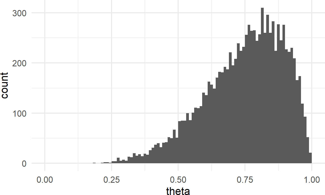
As a prior for a Bernoulli parameter, Figure 17.2 does seem valid in the sense that \(0 \leq \theta \leq 1\). Clearly however, this is not a uniform prior anymore. This prior suggests that values greater than \(50\%\) are much more likely than smaller values (i.e. there is more draws of higher theta values in the representative sample than lower theta values). So, to use this prior suggests that you have a strong prior belief that
success is more likely than failure.
17.2 Matching beta Parameters to Your Beliefs
With named probability distributions, we can use the stat_function layer available with ggplot to plot the exact distribution instead of the approximated distribution using a representative sample. For example, Figure 17.3 was made using the below code to plot the exact \(\textrm{beta}(6,2)\) distribution.
# create df with x-axis bounds
df = tibble(thetaBounds = c(0,1))

# initialize plot with bounds for x-axis
ggplot(df, aes(x=thetaBounds)) +
  stat_function(fun=dbeta,
                args = list(shape1 = 6, shape2 = 2))
Figure 17.3: The exact probability density function for a random variable with a beta(6,2) distribution.
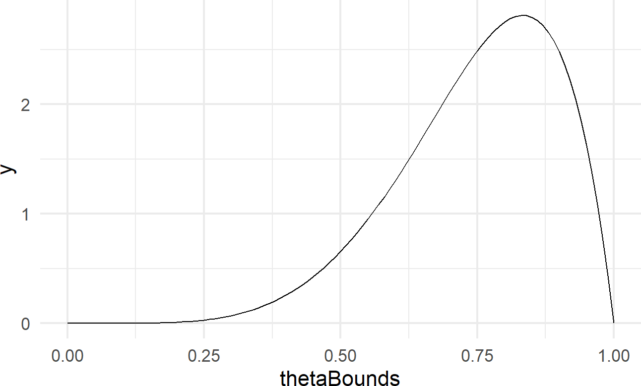
The function dbeta is an example of the
dfoo functions discussed in the Representing Uncertainty
chapter. For RV \(X\), it outputs the
probability density function, \(f(x)\)
for any given realization \(x\)
following a \(\textrm{beta(}\)shape1,shape2\(\textrm{)}\) distribution. Since the \(\textrm{beta}\) distribution is continuous,
we interpret higher density values as more probable and lower values as
less probable. Recall from your stats class, the area under the density
function represents probability and hence the area under any density
curve is exactly 1. See https://youtu.be/Fvi9A_tEmXQ from Khan Academy
for a refresher on probability density functions.
For most functions, stat_function is useful to get a quick visual. However, I prefer to use geom_area for probability density functions because the area under the curve represents probability and filling this area in with a color reminds us of this (see Figure 17.4 for example).
ggplot(df, aes(x=thetaBounds)) +
  geom_area(stat = "function",
            fun=dbeta,
            args = list(shape1 = 6, shape2 = 2),
            fill = "cadetblue")
Figure 17.4: Using geom area instead of stat function to plot a beta(6,2) distribution.
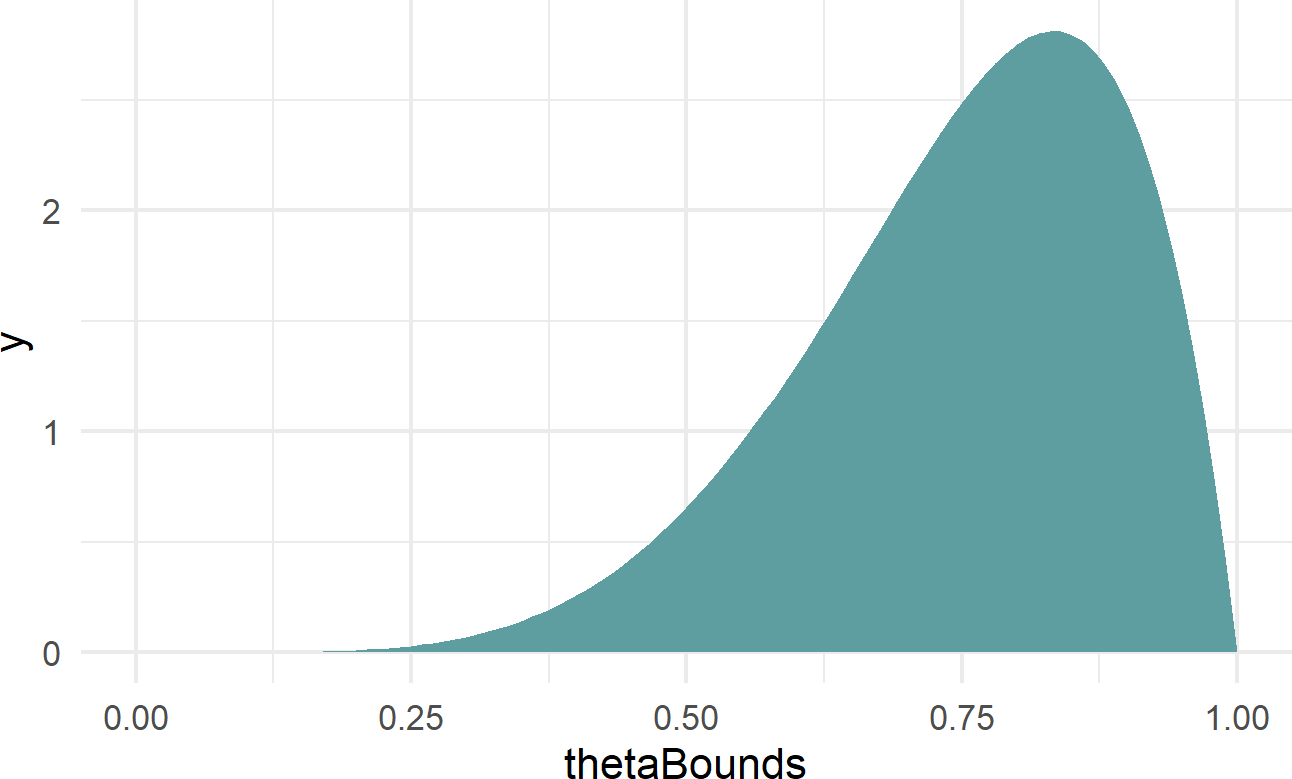
Figure 17.4 yields the same information as our representative sample shown in Figure 17.2; it just looks a little fancier. From the perspective of using the \(\textrm{beta}(6,2)\) to represent our beliefs about probability of success for a Bernoulli RV, we again see that higher probability values are more plausible than lower ones (i.e. there is more blue filled area above the higher theta values). If this represented our uncertainty in a trick coin’s probability of heads, we are suggesting that it is most likely biased to land on heads (i.e. more area for \(\theta\) values above 0.5 than below). That being said, there is visible area (i.e. probability) for the thetaBounds values below 0.5, so using this prior also suggests that the coin has the potential to be tails-biased; we would just need to flip the coin and see a bunch of tails to reallocate our plausibility beliefs to these lower values.
17.3 Investigating Various Parameters of The beta Distribution
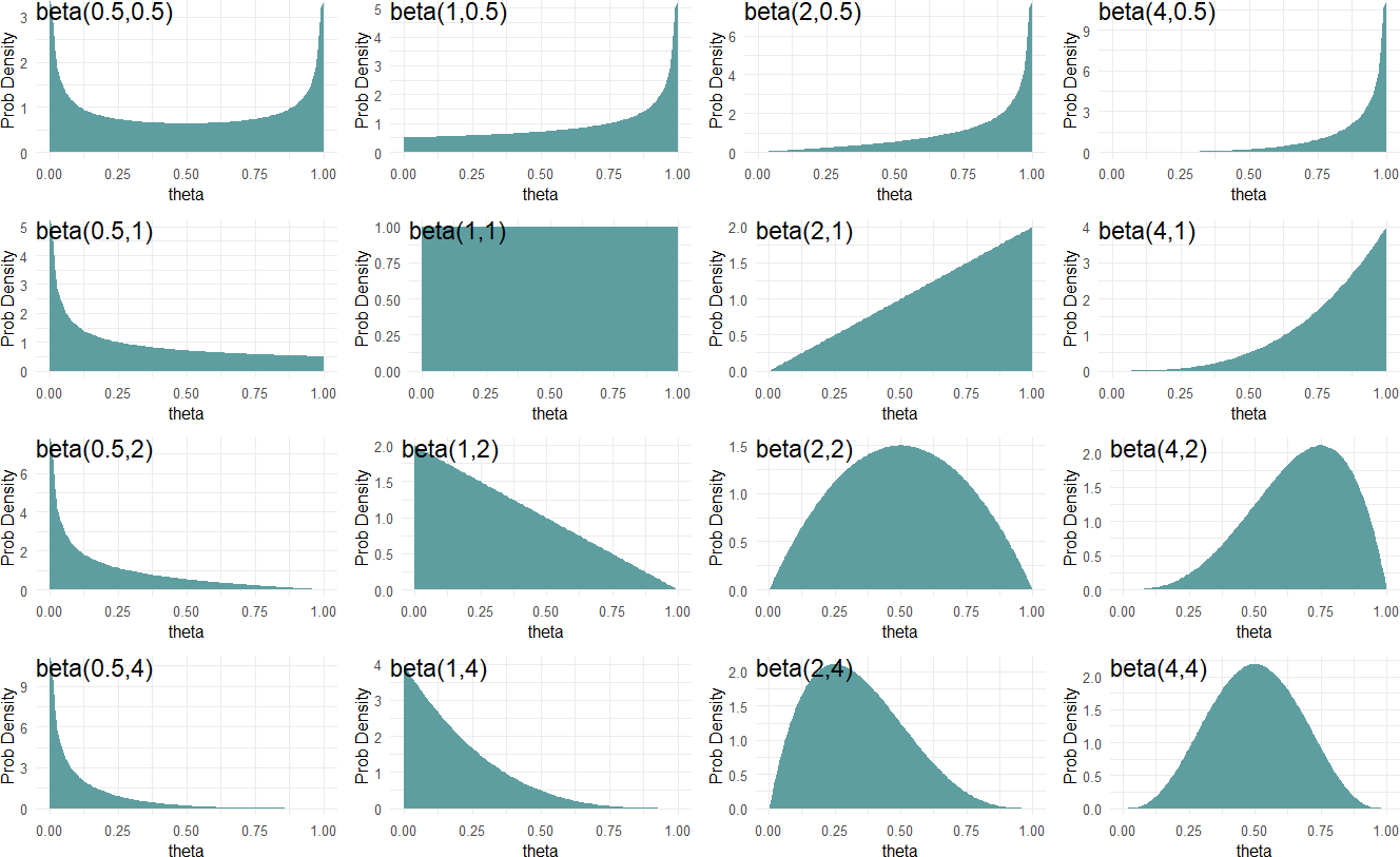
Figure 17.5: A diversity of beliefs about success probability can be modelled using different beta-distribution parameters.
Figure 17.5 shows beta distributions for various \(\alpha\) and \(\beta\) parameter values. From Figure 17.5, we see the \(\textrm{beta}\) distribution is flexible in showing a variety of representations of our uncertainty. When looking at the distribution for \(\textrm{beta}(0.5,0.5)\) (top-left) we see that theta values closer to zero or one have higher density values than values closer to 0.5. At the other end, a \(\textrm{beta}(4,4)\) distribution places more plausibility for values closer to 0.5. In between, it seems distributions that favor high or low values for \(\theta\) can be constructed.
\(^{**}\) See https://youtu.be/Fvi9A_tEmXQ for a refresher on continuous probability distributions.
The \(\textrm{beta}\) distribution has a very neat property which can aid your selection of parameters to model your uncertainty:
you can roughly interpret \(\alpha\) and \(\beta\) as previously observed data where the \(\alpha\) parameter is the number of successes you have observed and the \(\beta\) parameter is the number of failures.
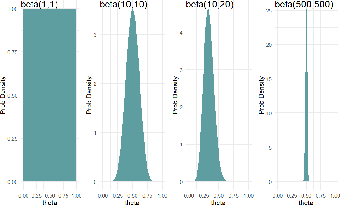
Hence, a \(\textrm{beta}(1,1)\) distribution\(^{**}\) can be thought of as saying a single success and failure have been witnessed, but we are completely unsure as to the probability of each. ** A beta(1,1) distribution is mathematically equivalent to a Uniform(0,1) distribution. Whereas, a \(\textrm{beta}(10,10)\) distribution is like suggesting you have seen 20 outcomes and they have been split down the middle - i.e. you have observed some small evidence that the two outcomes occur in equal proportions. Another distribution, say \(\textrm{beta}(10,20)\), can indicate a belief that would accompany having seen 30 outcomes where failures occur 2 times as frequently as successes. Finally, a distribution like \(\textrm{beta}(500,500)\) might be used to represent your uncertainty in the flip of a fair coin. Figure 17.6 shows these four distributions (i.e. probability density functions) side-by-side.
Figure 17.6: Comparing beta(1,1), beta(10,10), beta(10,20), and beta(500,500) distributions.
Moving forward, we will often use the \(\textrm{beta}\) distribution to represent our prior beliefs regarding a probability. The support is \((0,1)\) and it is able to adopt some flexible shapes. Take a moment and confirm that you can answer these thought questions:
THOUGHT Question: Let theta represent the probability of heads on a coin flip. Which distribution, beta(0.5,0.5), beta(1,1), beta(2,2), beta(50,100) or beta(500,500) best represents your belief in theta given that the coin is randomly chosen from someone’s pocket?
THOUGHT Question: Which distribution, beta(0.5,0.5), beta(1,1), beta(2,2), beta(50,100), or beta(500,500) best represents your belief in theta given the coin is purchased from a magic store and you have strong reason to believe that both sides are heads or both sides are tails?
17.4 Using a beta Prior
Let’s now use generative DAGs with the \(\textrm{beta}\) distribution to see how priors and data observations come together to make a posterior distribution.
Figure 17.7: Graphical model for Bernoulli data with a beta prior.
Figure 17.7 is a generative DAG declaring a \(\textrm{beta}(2,2)\) prior as representative of our uncertainty in \(\theta\). We aren’t saying too much with this prior. This is a weak prior because. as we will see, it will be easily overwhelmed by data; its just saying that two successes and two failures have been seen. Let’s imagine that we observe 20 successes and only two failures. This data is highly consistent with a very large value for theta. We can intelligently combine prior and data using dag_numpyro() to get our posterior:
# assume twenty successes and two failures
successData = c(rep(1,20),rep(0,2))

# get representative sample of posterior
graph = dag_create() %>%
  dag_node("Bernoulli RV","x",
           rhs = bernoulli(theta),
           data = successData) %>%
  dag_node("Bernoulli Parameter RV","theta",
           rhs = beta(2,2),
           child = "x")
drawsDF = graph %>% dag_numpyro()
And once the posterior sample (drawsDF) is created, we can query the results and compare them to the \(\textrm{beta}(2,2)\) prior:
library(tidyverse)

# named vector mapping colors to labels
colors = c("beta(2,2) Prior" = "aliceblue",
           "Posterior" = "cadetblue")

# use geom_density to create smoothed histogram
ggplot(drawsDF, aes(x = theta)) +
  geom_area(stat = "function", fun = dbeta,
            args = list(2,2),
            alpha = 0.5, color = "black",
            aes(fill = "beta(2,2) Prior"))+
  geom_density(aes(fill = "Posterior"),
               alpha = 0.5) +
  scale_fill_manual(values = colors) +
  labs(y = "Probability Density",
       fill = "Distribution Type") +
  xlim(0,1)
Figure 17.8: Posterior distribution is right-shifted from the beta(2,2) prior distribution after observing data with 20 successes and 2 failures.
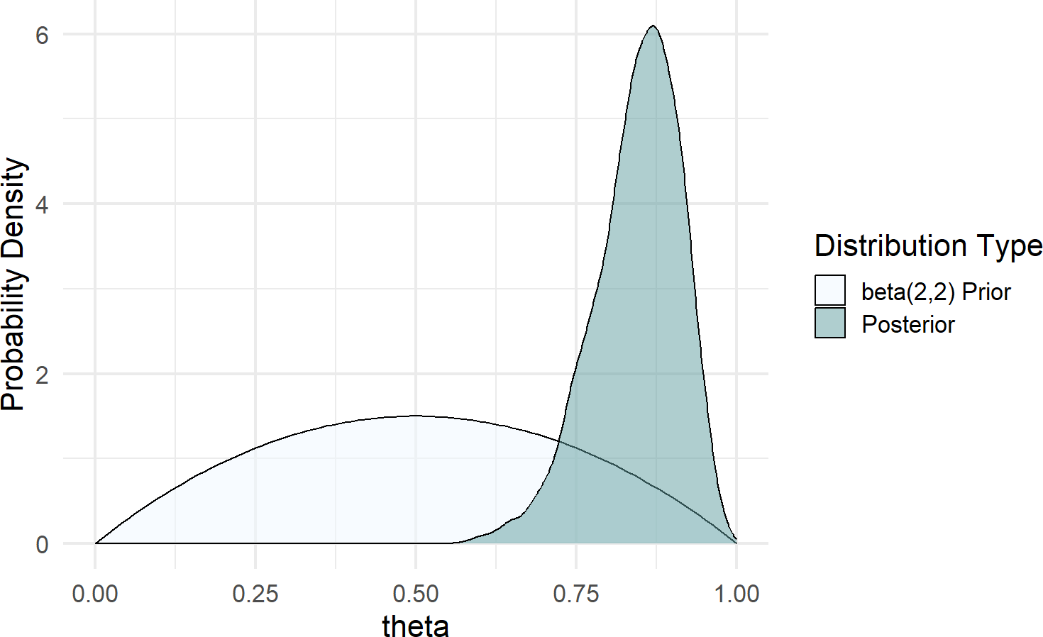
Figure 17.8 shows a dramatic shift from prior to posterior distribution. The weak prior suggested ot us that all values between zero and one had plausibility, but once observing 20 successes out of 22 trials, the higher values for \(\theta\) became much more plausible.
If we want to change the prior to something stronger, say a \(\textrm{beta}(50,50)\), then we can rerun dag_numpyro() after just changing the one line for the prior:
graph = dag_create() %>%
  dag_node("Bernoulli RV","x",
           rhs = bernoulli(theta),
           data = successData) %>%
  dag_node("Bernoulli Parameter RV","theta",
           rhs = beta(50,50),  ### UPDATED FOR NEW PRIOR
           child = "x")

drawsDF = graph %>% dag_numpyro()Figure 17.9: Posterior distribution is right-shifted from the beta(2,2) prior distribution after observing data with 20 successes and 2 failures.
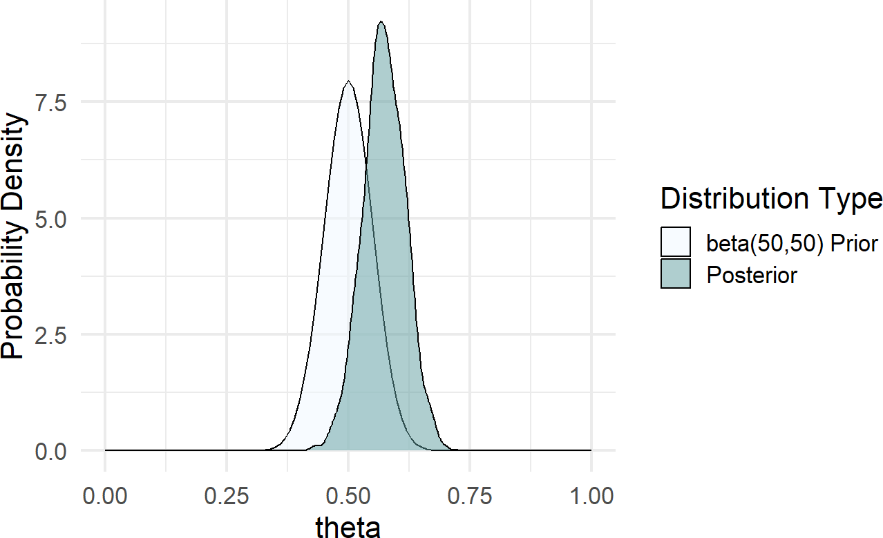
Figure 17.9 shows a posterior distribution that is only mildly shifted from its prior. This is a direct result of a strong prior due to the larger \(\alpha\) and \(\beta\) parameters. In general, we will seek weakly informative priors that yield plausible prior generating processes, yet are flexible enough to let the data inform the posterior generating process. There is a bit of an art to this and we will learn more in subsequent chapters.
17.5 Exercises
Figure 17.10 shows the generative DAG to be used in answering the following exercises:
Figure 17.10: A generative DAG for the results of a taste testing survey.
Your company has been testing two flavors of coffee using free samples, let’s call them Flavor A and Flavor B. You are planning to only offer one flavor for sale and are interested in whether your customers prefer Flavor A or Flavor B.
You use a taste testing survey of 60 randomly selected people, and find that 36 people prefer Flavor B.
Exercise 17.1 Using causact and assuming the generative DAG of Figure 17.10, determine the posterior probability that Flavor B is preferred to Flavor A. In other words, what percentage of your posterior draws have a theta that is above 0.5?
Exercise 17.2 You use a taste testing survey of 600 randomly selected people, and find that 360 people prefer Flavor B.
Using causact and assuming the generative DAG of Figure 17.10, determine the posterior probability that Flavor B is preferred to Flavor A. In other words, what percentage of your posterior draws have a theta that is above 0.5?